Radiation model calibration

Description

This text describes how to calibrate the radiation model P1CFDEM using the result from a test consisting of a particle bed being compacted between two parallel horizontal plates. The bottom plate is kept at a constant temperature, while the top one is subjected to a constant heat flux; see Figure 1.

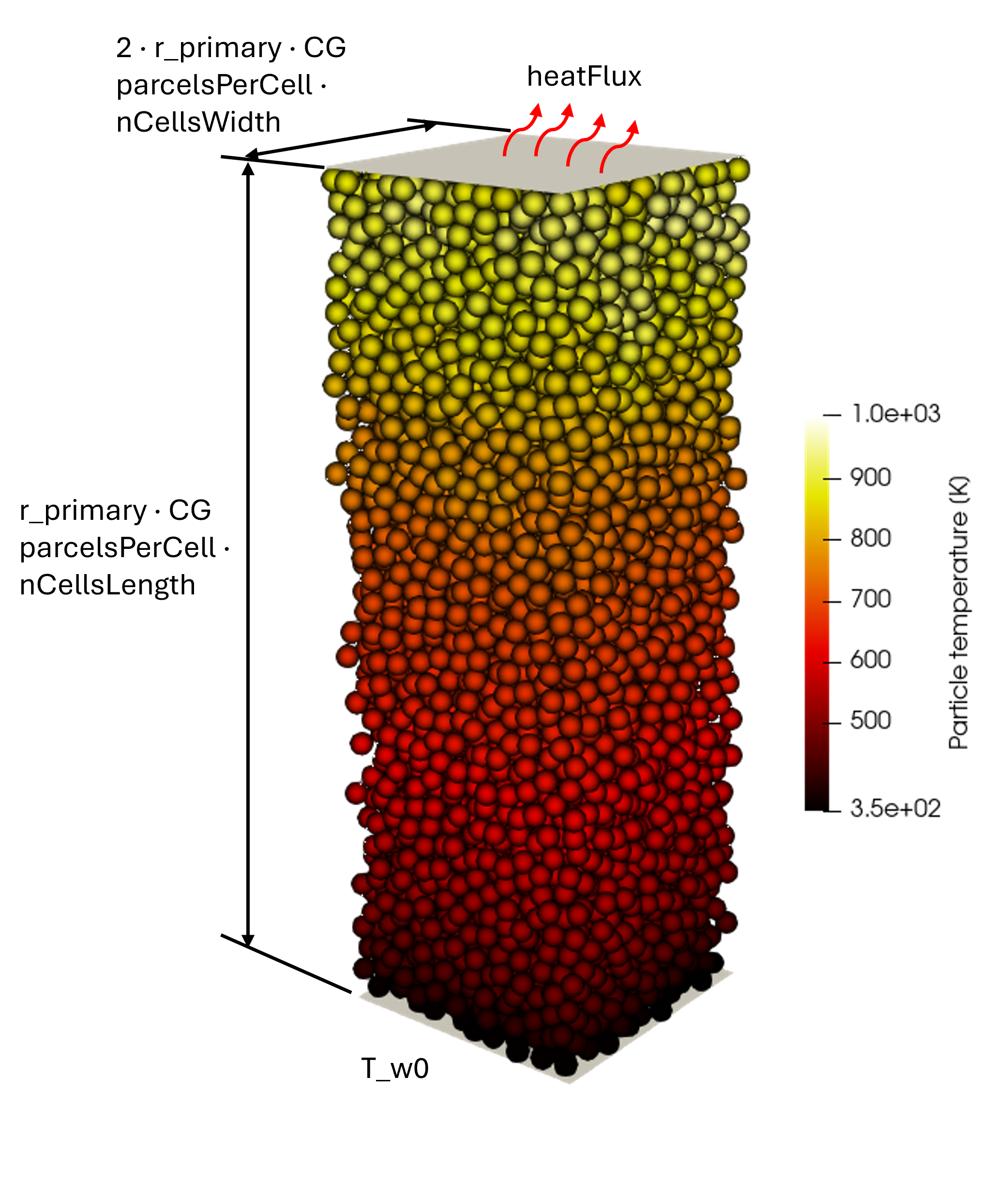
Figure 1: tutorial’s simulation setup

Introduction

This tutorial shows an application of the template heatTransferRadiation, which has been developed to calibrate the P1 radiation model described in Mačak et al..

The setup consists of a square prism filled with spherical particles. The top and bottom of the container are solid plates, while the lateral boundary conditions are periodic. The top plate compresses the bulk material with a normal pressure equal to sigma_n until reaching a steady-state.

After the consolidation phase is concluded, a constant temperature and heat flux are imposed at the bottom and top plate, respectively. At each calibration iteration, the effective heat transfer coefficient is calculated and compared to the reference one. The material properties calibrated in this tutorial are the particle emissivity epsilon_p, the particle absorption efficiency Qabs_p, and the particle scattering efficiency Qsca_p. The coefficient triplet returning the best agreement between reference and simulated data represents the solution of the calibration.

Detailed descriptions

Contact model and coarsegraining factor

The contact model used by the template is hardcoded and equal to the Hertz normal and the tangential history.

The coarsegraining factor is defined in the input file radiationHeatTransfer.casx under CG and set equal to 1.

Material properties and particle size distribution

The values of the fixed material parameters and the initial, minimum and maximum values of the target material parameters, as well as the particle size distribution, are defined in the file radiationHeatTransfer.casx.

Calibration case settings

The tutorial consists of one calibration_case of the template heatTransferRadiation. More information about the template-specific settings of the calibration case can be found in the relative documentation.

Running the tutorial and analyzing the results

The user can run the tutorial via command line as follows:

aspherix-calibration run -in radiationHeatTransfer.casx -skip-qf-check true

The skip-qf-check true command-line option is needed beacuse the quality function of the corresponding calibration template is defined directly in the Aspherix solver input scripts.

The case will run by default using 4 cores. The convergence of the calibration is reported in the file calibration/results/conv.dat, which reads as follows:

# nIter           Qabs_p           Qsca_p        epsilon_p         qf_total
      1              0.5              0.5              0.5          6.34641
      3         0.166667              0.5              0.5          2.38895
      8         0.166667         0.833333              0.5          1.40205
     17        0.0555556         0.833333         0.833333         0.809835
     25        0.0555556         0.722222         0.833333         0.740253
     39        0.0185185         0.722222         0.944444         0.374473
     46        0.0185185         0.759259         0.944444         0.366406
     61       0.00617284         0.759259         0.981481        0.0540793
     72       0.00617284         0.771605         0.981481        0.0522953

The iteration returning the lowest value of the quality function is the number 72, which corresponds to a relative error between the reference and simulated effective heat transfer coefficient of around 5%.

[1] J. Mačak, C. Goniva, St. Radl (2023). “Predictions of the P1 approximation for radiative heat transfer in heterogeneous granular media” Particuology 82: 25-47.