Create a user-template

Description

This article describes how to create from scratch a template for calibrating the powder flowability using a powder flow tester.

Step 1: creation of the simulation setup

The simulaton of the powder flow tester can divided into a filling phase and a discharging phase; see Figure 1. During the filling phase, a closed cylinder is filled with a certain mass of powder, while during the discharging phase, the bottom lid of the cylinder is removed and the powder flows outside the cylinder. During the discharging phase, the mass of the powder inside the cylinder is written to file every time interval. The calibration occurs by iteratively changing the rolling friction coefficient and by comparing the discharge curve obtained from the simulation with a reference one.

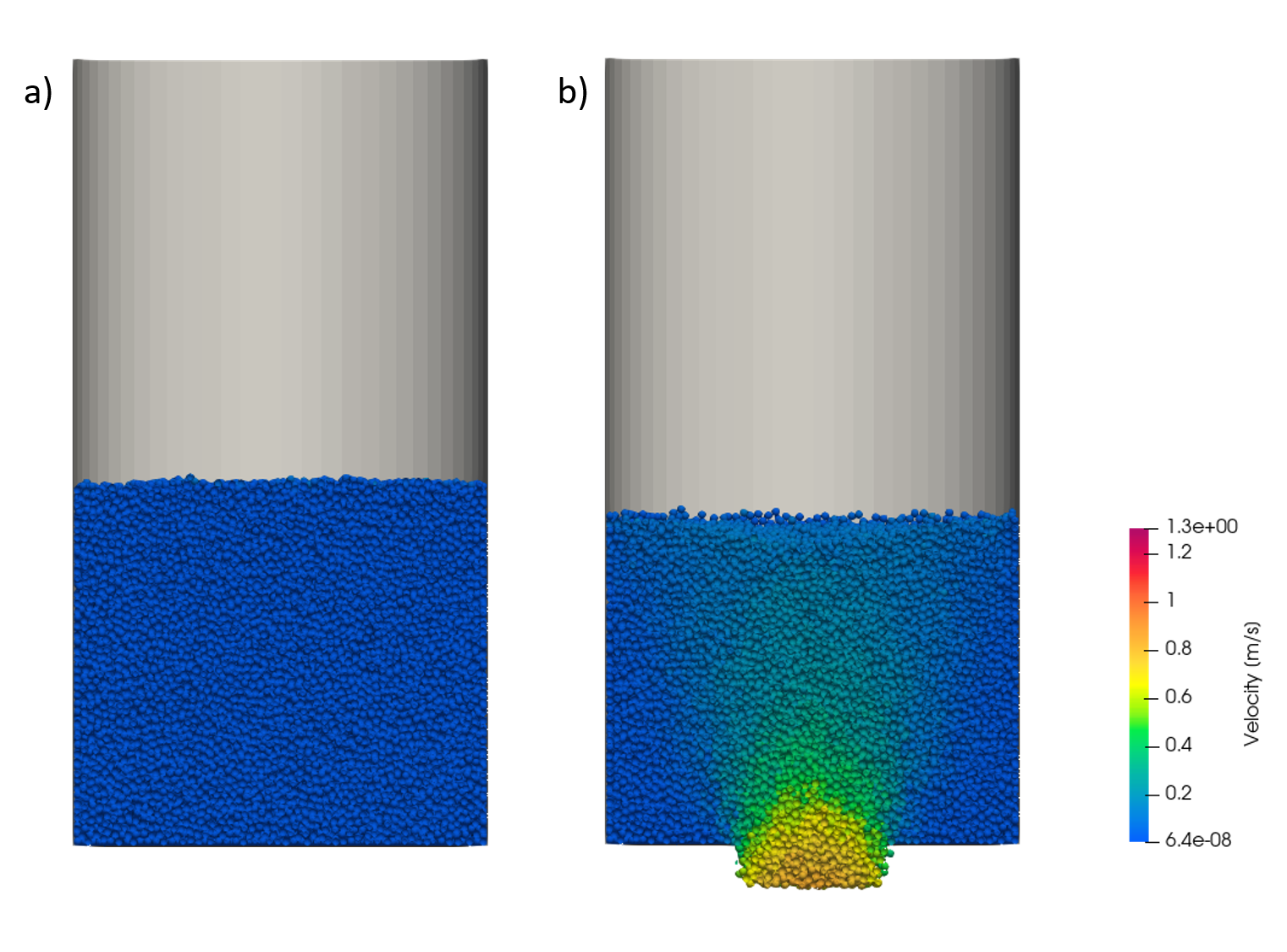
Figure 1: Simulation of a) filling phase and b) discharging phase.

The filling and discharding phase simulations are encapsulated into two distinc Aspherix® input scripts, namely init.asx and run.asx. Both input scripts, generated using Aspherix® GUI, are reported here:

# Filling phase (init.asx)
particle_shape sphere
simulation_domain low ( -0.05, -0.05, 0 ) high ( 0.05, 0.05, 0.2 )
simulation_timestep 1e-5
write_output_timestep 0.01
write_to_terminal_timestep 0.01
materials { particle, wall }
region reg1 cylinder center_bottom ( 0, 0, 0.01 ) center_top ( 0, 0, 0.2 ) radius 0.05
material_interaction_properties wall particle coefficientFriction 0.2 coefficientRestitution 0.2 coefficientRollingFriction 0.2
material_properties particle coefficientFriction 0.1 coefficientRestitution 0.1 coefficientRollingFriction 0.1 density 1200 poissonsRatio 0.3 youngsModulus 1e7
material_properties wall coefficientFriction 0.1 coefficientRestitution 0.1 coefficientRollingFriction 0.1 density 2000 poissonsRatio 0.3 youngsModulus 1e8
particle_contact_model normal hertz tangential history cohesion off rolling_friction epsd2 settings
wall_contact_model normal hertz tangential history cohesion off rolling_friction epsd2 settings
primitive_wall id pw1 material wall type cylinder center_bottom ( 0, 0, 0.01 ) center_top ( 0, 0, 0.2 ) radius 0.05
primitive_wall id pw2 material wall type disk center ( 0, 0, 0.01 ) normal ( 0, 0, 1 ) radius 0.05 inner_radius 0.02
primitive_wall id pw3 material wall type disk center ( 0, 0, 0.01 ) normal ( 0, 0, 1 ) radius 0.02
particle_template id pt1 material particle shape sphere radius 0.001
particle_distribution id pd1 templates { pt1 } fractions { 1 } seed 1804289383
insertion mode pack region reg1 target_mass 0.5 particle_distribution pd1 velocity constant ( 0, 0, -1 ) id ins1
check_timestep
enable_gravity
enable_loadbalancing
output_settings
simulate mode until_settled
write_restart restart/restart.latest

# Discharging phase (run.asx)
particle_shape sphere
read file restart/restart.latest reset_timestep yes
simulation_domain low ( -0.05, -0.05, 0 ) high ( 0.05, 0.05, 0.2 )
simulation_timestep 1e-5
write_output_timestep 0.01
write_to_terminal_timestep 0.01
materials { particle, wall }
region reg1 cylinder center_bottom ( 0, 0, 0.01 ) center_top ( 0, 0, 0.2 ) radius 0.05
material_interaction_properties wall particle coefficientFriction 0.2 coefficientRestitution 0.2 coefficientRollingFriction 0.2
material_properties particle coefficientFriction 0.1 coefficientRestitution 0.1 coefficientRollingFriction 0.1 density 1200 poissonsRatio 0.3 youngsModulus 1e7
material_properties wall coefficientFriction 0.1 coefficientRestitution 0.1 coefficientRollingFriction 0.1 density 2000 poissonsRatio 0.3 youngsModulus 1e8
particle_contact_model normal hertz tangential history cohesion off rolling_friction epsd2 settings
wall_contact_model normal hertz tangential history cohesion off rolling_friction epsd2 settings
primitive_wall id pw1 material wall type cylinder center_bottom ( 0, 0, 0.01 ) center_top ( 0, 0, 0.2 ) radius 0.05
primitive_wall id pw2 material wall type disk center ( 0, 0, 0.01 ) normal ( 0, 0, 1 ) radius 0.05 inner_radius 0.02
particle_template id pt1 material particle shape sphere radius 0.001
particle_distribution id pd1 templates { pt1 } fractions { 1 } seed 1804289383
check_timestep
enable_gravity
enable_loadbalancing
calculate sum quantity mass particle_group all region reg1 id cal1
output_settings
workbench_custom_command write_to_file string "id_time id_cal1" file mass.txt
workbench_custom_command simulate time 0.5
simulate mode until_settled

Step 2: creation of the case.conf file

The case.conf file contains essentially three classes of settings:

• general template setting

• specific template setting

• run settings for the calibration workflow

The general template settings include contact models, number of processors, and output settings. An extensive list can be found here. The specific settings, on the other hand, strictly depend on the template we aim to develop. In case of a powder flow tester template, the following specific settings can be identified:

• radius of the bottom orifice r_hole

• radius of the cylindrical vessel r_silo

• height of the vessel h_silo

• powder mass mass

While the geometrical parameters should have a defaul value (as they might refer to a specific experimental setup), the powder mass should be kept undefined.

The run settings determines which input script is the initialization one, which one(s) belongs to the calibration cycle, and whether the scripts are run in serial or in parallel. Another run setting (not used here) allows to specify an already existing quality function for the user template; please, see qualityFcnType documented here.

The case.conf file could read as follows:

# Case settings for the flow tester
# mpi
NPROC 4
# models
pairGranModel hertz
pairTangential history
pairCohesion off
pairRollingFriction epsd2
pairSurface default
# dump settings
dumpT 0.01
dump 0
# Default parameters for the calibration_case command
r_hole 0.02
r_silo 0.05
h_silo 0.2
mass *undefined*
# Run mode settings
runMode "direct"
initDirectModes "mpi"
initDirectScripts "init.asx"
runDirectModes "mpi"
runDirectScripts "run.asx"

Step 3: modification of the simulation input files

Some of the strings and numerical quantities defined in the init.asx and run.asx input files need to be replaced by variables in order to make the simulation workflow as generic as possible. The settings contained in the case.conf file, together with additional ones which are automatically calculated (e.g., the DEM time-step DEMts), are loaded from the caseVariables file. This file is generated automatically by Aspherix® Calibration and is located inside the simulation folder.

The material parameters, both fixed and calibrated, are contained in the optimVariables file, which is also generated automatically by Aspherix® Calibration. The path of the optimVariables file is either ../../../temp/optimVariables (for the initialization simulation) or ../../optimVariables, both relative to the simulation folder. The material parameters that are generally required are reported here.

The particle template(s) and size distribution are automatically created by Aspherix® Calibration based on the calibration input script (see particle_template command and particle_distribution command). The information about the particle template(s) and size distribution is contained in the aspherixPartDist.txt file, which has to be included in the init.asx file. The ID of the particle distribution in the aspherixPartDist.txt file is hardcoded to pdd1 and the particle material name is particle.

Finally, the quality function is calculated by calling a Python script in the run.asx input file using the shell command.

Both modified input scripts are reported here:

# Filling phase (init.asx)
include_foam_variables caseVariables
include_foam_variables ../../../temp/optimVariables
particle_shape sphere
variable z_max equal 0.01+${h_silo} # 0.01 is the hardcoded z-coordinate of the silo's bottom
simulation_domain low ( -${r_silo}, -${r_silo}, 0 ) high ( ${r_silo}, ${r_silo}, ${z_max} )
simulation_timestep ${DEMts}
write_output_timestep ${dumpT}
write_to_terminal_timestep ${dumpT}
materials { particle, wall }
region reg1 cylinder center_bottom ( 0, 0, 0.01 ) center_top ( 0, 0, ${z_max} ) radius ${r_silo}
material_interaction_properties wall particle coefficientFriction ${c_frict_pw} coefficientRestitution ${c_rest_pw} coefficientRollingFriction ${c_rollFrict_pw}
material_properties particle coefficientFriction ${c_frict_pp} coefficientRestitution ${c_rest_pp} coefficientRollingFriction ${c_rollFrict_pp} density ${rho_p} poissonsRatio ${poissonsR_p} youngsModulus ${Y_p}
material_properties wall coefficientFriction ${c_frict_pw} coefficientRestitution ${c_rest_pw} coefficientRollingFriction ${c_rollFrict_pw} density ${rho_w} poissonsRatio ${poissonsR_w} youngsModulus ${Y_w}
particle_contact_model normal ${pairGranModel} tangential ${pairTangential} cohesion ${pairCohesion} rolling_friction ${pairRollingFriction}
wall_contact_model normal ${pairGranModel} tangential ${pairTangential} cohesion ${pairCohesion} rolling_friction ${pairRollingFriction}
primitive_wall id pw1 material wall type cylinder center_bottom ( 0, 0, 0.01 ) center_top ( 0, 0, ${z_max} ) radius ${r_silo}
primitive_wall id pw2 material wall type disk center ( 0, 0, 0.01 ) normal ( 0, 0, 1 ) radius ${r_silo} inner_radius ${r_hole}
primitive_wall id pw3 material wall type disk center ( 0, 0, 0.01 ) normal ( 0, 0, 1 ) radius ${r_hole}
# Load particle templates
include aspherixPartDist.txt
insertion mode pack region reg1 target_mass ${mass} particle_distribution pdd1 velocity constant ( 0, 0, -1 ) id ins1
check_timestep
enable_gravity
enable_loadbalancing
output_settings
if "${dump} == 1" then &
    "output_settings write_every_time ${dumpT}" &
else "print 'no dumps activated'"
simulate mode until_settled
write_restart restart/restart.latest

# Discharging phase (run.asx)
include_foam_variables caseVariables
include_foam_variables ../../optimVariables
particle_shape sphere
read file restart/restart.latest reset_timestep yes
variable z_max equal 0.01+${h_silo} # 0.01 is the hardcoded z-coordinate of the silo's bottom
simulation_domain low ( -${r_silo}, -${r_silo}, 0 ) high ( ${r_silo}, ${r_silo}, ${z_max} )
simulation_timestep ${DEMts}
write_output_timestep ${dumpT}
write_to_terminal_timestep ${dumpT}
materials { particle, wall }
region reg1 cylinder center_bottom ( 0, 0, 0.01 ) center_top ( 0, 0, ${z_max} ) radius ${r_silo}
material_interaction_properties wall particle coefficientFriction ${c_frict_pw} coefficientRestitution ${c_rest_pw} coefficientRollingFriction ${c_rollFrict_pw}
material_properties particle coefficientFriction ${c_frict_pp} coefficientRestitution ${c_rest_pp} coefficientRollingFriction ${c_rollFrict_pp} density ${rho_p} poissonsRatio ${poissonsR_p} youngsModulus ${Y_p}
material_properties wall coefficientFriction ${c_frict_pw} coefficientRestitution ${c_rest_pw} coefficientRollingFriction ${c_rollFrict_pw} density ${rho_w} poissonsRatio ${poissonsR_w} youngsModulus ${Y_w}
particle_contact_model normal ${pairGranModel} tangential ${pairTangential} cohesion ${pairCohesion} rolling_friction ${pairRollingFriction}
wall_contact_model normal ${pairGranModel} tangential ${pairTangential} cohesion ${pairCohesion} rolling_friction ${pairRollingFriction}
primitive_wall id pw1 material wall type cylinder center_bottom ( 0, 0, 0.01 ) center_top ( 0, 0, ${z_max} ) radius ${r_silo}
primitive_wall id pw2 material wall type disk center ( 0, 0, 0.01 ) normal ( 0, 0, 1 ) radius 0.05 inner_radius ${r_hole}
check_timestep
enable_gravity
enable_loadbalancing
calculate sum quantity mass particle_group all region reg1 id cal1
if "${dump} == 1" then &
    "output_settings write_every_time ${dumpT}" &
else "print 'no dumps activated'"
workbench_custom_command write_to_file string "id_time id_cal1" file mass.txt
simulate mode until_settled
workbench_custom_command simulate time 0.5
shell ./calculate_qf.py

Step 4: calculation of the quality function

In case the user-template does not rely on an existing quality function, Aspherix® Calibration expects after each iteration a file named Fun.txt inside the simulation folder, which contains single floating point number in ASCII format. This number, which is interpreted as the user-template quality function, must quantify the difference between a simulated and a reference observable. In this tutorial, we consider the quality function to be equal to the distance between the simulated and reference discharge curves. The discharge curve is defined as the mass of powder inside the container as a function of time.

The script calculate_qf.py is reported below:

#! /usr/bin/python3

import numpy as np
import math
from scipy import interpolate

inputRef = (np.loadtxt('reference.txt'))
inputSim = (np.loadtxt('mass.txt'))

inputSim_int = interpolate.interp1d(inputSim[:,0], inputSim[:,1], kind='linear', fill_value= 'extrapolate')
inputSim_new = np.zeros((len(inputRef),2))

for i in range(np.shape(inputRef)[0]):
    inputSim_new[i,0] = inputRef[i,0]
    inputSim_new[i,1] = inputSim_int(inputRef[i,0])

outputFile = open('Fun.txt','w')
outputFile.write("%10.10f" % (math.dist(inputRef[:,1],inputSim_new[:,1])))
outputFile.close()

Step 5: user-template folder structure

The files init.asx, run.asx, case.conf and calculate_qf.py must be contained in a folder named after the template, e.g., powderFlowTester. The powderFlowTester folder, in turn, must be located inside a folder named Aspherix. The location of the Aspherix can be decided arbitrarily by the user.

Step 6: creation of a calibration case

The user-template can be tested by using the following calibration input script:

# 1) FIXED PARAMETERS (they do NOT change during calibration)
param_fixed coarsegraining type scalar value 1.0
param_fixed Y_w type scalar value 1e8
param_fixed Y_p type scalar value 1e7
param_fixed poissonsR_w type scalar value 0.3
param_fixed poissonsR_p type scalar value 0.3
param_fixed c_rest_pw type scalar value 0.2
param_fixed c_rest_pp type scalar value 0.1
param_fixed c_frict_pp type scalar value 0.1
param_fixed c_frict_pw type scalar value 0.2
param_fixed c_rollFrict_pw type scalar value 0.01
param_fixed rho_p type scalar value 1200
param_fixed rho_w type scalar value 2000

# 2) TARGET PARAMETERS (they DO change during calibration)
param_calibration c_rollFrict_pp type linear init 0.1 min 0.01 max 0.2

# 3) PARTICLE DISTRIBUTION
particle_template pt1 shape sphere radius 0.001
particle_distribution p templates pt1 mass_fractions 1

# 4) SYSTEM SETTINGS (to override settings in etc/dalilama.conf)

# 5) OPTIMIZER SETTINGS
optimizer_setting maxFunctionEval 20

# 6) CALIBRATION SETUP

# Inclination test
calibration_case test1 template powderFlowTester type Aspherix target_param c_rollFrict_pp     &
    measfile measurements/flow_curve.txt parameter_overrides                                   &
    mass                0.5                                                                    &
    dump                1                                                                      &
    dumpT               0.01                                                                   &
    NPROC               4

# 7) RUN CALIBRATION
run single

The only parameter that is calibrated is the rolling friction coefficient between particles. The reference discharding curve is contained in the file measurements/flow_curve.txt. The flow_curve.txt files reads as follows:

0.00 0.500
0.50 0.300
1.00 0.123
1.50 0.064
2.00 0.050
2.50 0.043

Step 7: launching the calibration

To start the calibration, the user should use the following command:

aspherix-calibration run -in powder_flow_tester.casx -user-template-dir /path_to_user_template

where powder_flow_tester.casx is the name of the Aspherix® Calibration input script defined in the previous section, and /path_to_user_template is the path to the folder hosting the Aspherix folder (in which the new template powderFlowTester is contained).

Step 8: analyzing the results

The convergence of the calibration is reported in the file calibration/results/conv.dat, which reads as follows:

# nIter   c_rollFrict_pp         qf_total
  1            0.105        0.0175081
  5        0.0838889        0.0146419
  6        0.0627778        0.0116733

The iteration returning the lowest value of the quality function is the number 6. The comparison between the reference and the simulated yield locus is shown in Figure 2.

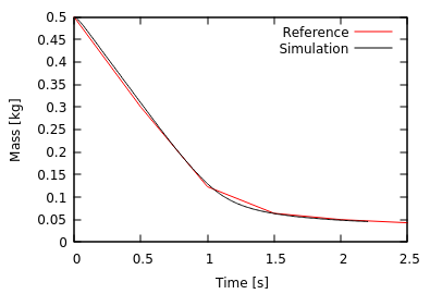
Figure 2: discharging curve (reference and simulation 6).