Rotating drum test

Description

This tutorial describes how to calibrate the particle-particle (p-p) static and rolling friction coefficients using a rotating drum test.

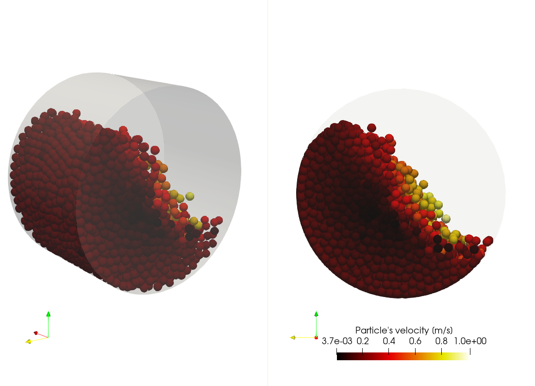
Figure 1: result obtained from the rotatingDrum tutorial.

Introduction

This tutorial shows an application of the calibration template rotaryDrum. The setup consits of a cylindrical drum half filled with spherical particles. After the particle insertion and settling phases, the drum starts rotating with the prescribed velocity of 32 RPM. After an initial transient of 0.5 s, images of the simulation are taken over a time span of 0.5 s and used to calculate the average inclination of the interface. This value is then compared to the reference reported in the file measurements/rotatingDrum.dat. During the calibration process, different values of the p-p static and rolling friction coefficients are selected within a prescribed range. The coefficient values returning the best agreement between simulation and reference (i.e., lowest value of the quality function) represent the solution of the calibration.

Detailed descriptions

Contact model and coarsegraining factor

The contact model and the coarsegraining factor are defined in the file settings/contact_model.txt. The models used in this tutorial are: Hertz normal, tangential history, rolling friction epsd. The cohesion model is switched off and the surface model is set to default. More information about the contact models allowed by the rotating drum template can be found here. The calibration simulations are performed with a coarsegraining factor 1.5.

Material properties and particle size distribution

The values of the fixed material parameters and the initial, minimum and maximum values of the target material parameters are defined in the file settings/materials.txt.

Warning

Not all the parameters specified in materials.txt are used by the simulations, as it depends on the contact models selected in contact_model.txt

The particle size distribution is defined in the file settings/particle_sizes.txt.

Calibration case settings

The tutorial consists of a single calibration_case of the template rotatingDrum. Some template-specific settings of the calibration case are defined in the file settings/tests.txt. These include the sizes of the drum (radius and length), rotation rate, filling level, etc. Other more general settings, like the number of iterations of the calibration procedure, can be found in the file settings/general.txt.

Running the tutorial and analyzing the results

The user can run the tutorial via command line as follows:

aspherix-calibration run -in rotating_drum.casx

The convergence of the calibration is reported in the file calibration/results/conv.dat, which reads as follows:

# nIter       c_frict_pp   c_rollFrict_pp      qf_total
  1            0.405            0.405          3.23067
  2            0.668333         0.405          2.28017
 11            0.580556         0.405          1.04303

The iteration returning the lowest value of the quality function is the number 11. In this case, the average inclination of the interface obtained from the simulation is around 49 deg, while the reference is 50 deg.

Figure 2 shows in blue the average interface profile and in green plus/minus the standard deviation of the interface profile. This picture is automatically generated by Aspherix® Calibration and can be found in each working directory under the name result.png (the exact path is calibration/workDir/workDir.X/Aspherix/test1/result.png).

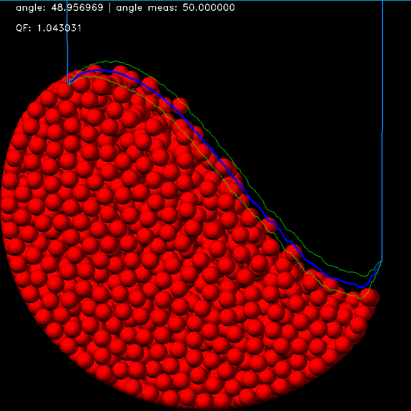
Figure 2: average (blue line) and standard deviation (green line) of the interface profile for iteration 11.

Calibration with multispheres

The used can substitute spherical particles with multispheres by changing the rotating_drum.casx input file as follows:

particle_template p1 shape multisphere file ms.txt
#particle_template p1 shape sphere radius ${rp1}
particle_distribution p templates p1 mass_fractions ${mf1}

The shape of the multisphere is defined in the file ms.txt. Each line corresponds to a particle forming the multisphere, while the columns contain, in order, the x, y, z coordinates of the particle center and its radius.

The results of the calibration is once again summarized by the file calibration/results/conv.dat:

# nIter       c_frict_pp   c_rollFrict_pp         qf_total
      1            0.405            0.405          3.98011
     10            0.405         0.492778          3.78053
     15         0.317222         0.492778          3.53478
     22         0.317222         0.522037           3.3047

The best agreement match between simulation and reference data is obtained at the 22th iteration, although the quality function here is not as low as the case with spheres. In this case, the average inclination of the interface obtained from the simulation is around 46.7 deg, while the reference is 50.0 deg. Figure 3 shows in blue the average interface profile and in green plus/minus the standard deviation of the interface profile.

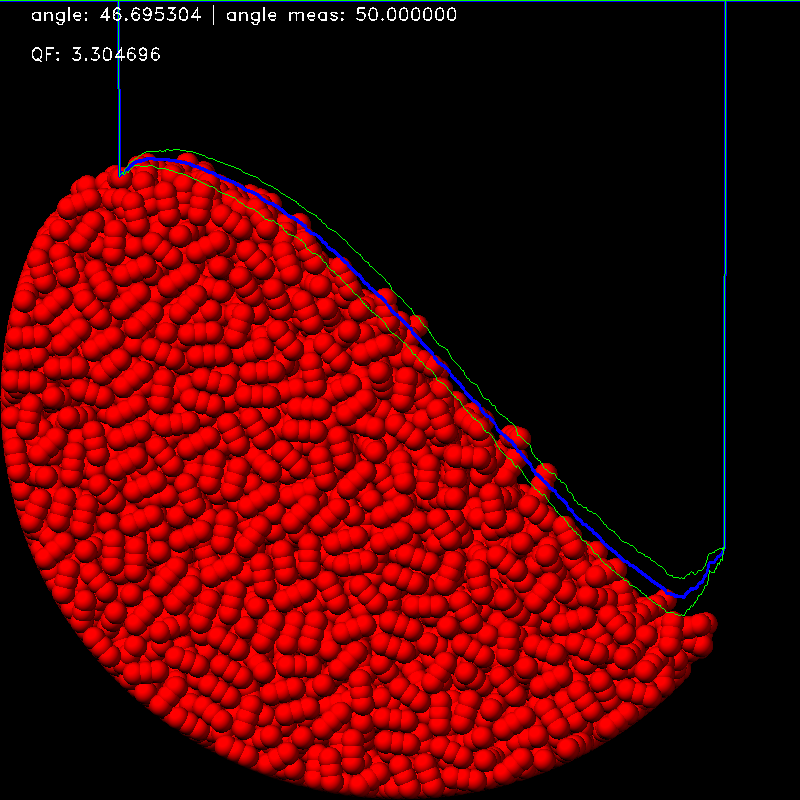
Figure 3: average (blue line) and standard deviation (green line) of the interface profile for iteration 22.