 Home
HomeViscoelastic model calibration
Description
This text describes how to calibrate the DEM model for a viscoelastic paste using results from a rotational rheometer.
Introduction
This tutorial shows an application of the calibration template
oscillatoryRheometerBurgers.
The setup consists of a laterally-unconfined cubic lattice of
spherical particles which undergoes periodic shear in the horizontal
plane. The height of the lattice is equal to 10 particle’s diameters; see
Figure 1. The amplitude of the oscillation,  , is set equal to
5% of the lattice’s height,
, is set equal to
5% of the lattice’s height,  . The frequencies of the oscillations
are:
. The frequencies of the oscillations
are:  ,
,  and
and
 .
.
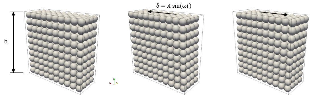
Figure 1: particle lattice undergoing periodic shearing.
The scope of this tutorial is to calibrate the asphalt tangential contact model so that the viscosity of the model material corresponds to the reference value over a certain interval of frequencies.
Detailed descriptions
Contact model
The contact model and the coarsegraining factor are defined in the file
settings/contact_model.txt. The models used in this tutorial are:
Hertz normal contact, asphalt
tangential contact, asphalt cohesion model.
Material properties and particle size distribution
The values of the fixed material parameters and the initial, minimum and
maximum values of the target material parameters are defined in
the file settings/materials.txt.
Warning
Not all the parameters specified in materials.txt are used
by the simulations, as it depends on the contact models selected
in contact_model.txt
The particle size distribution is defined in the file
settings/particle_sizes.txt.
Calibration case settings
The tutorial consists of a single calibration_case of the
template oscillatoryRheometerBurgers.
Some template-specific settings of the calibration case are defined in the file
settings/tests.txt.
Other more general settings, like the number of iterations of the calibration procedure,
can be found in the file settings/general.txt.
Running the tutorial and analyzing the results
The user can run the tutorial via command line as follows:
aspherix-calibration run -in viscoelastic_calibration.casx
The convergence of the calibration is reported in the file
calibration/results/conv.dat, which reads as follows:
# nIter kelv_nu maxw_Y qf
  1        50500      550000    0.856388
  2        83500      550000    0.285046
  6        83500      850000    0.147139
 10        94500      850000   0.0407045
 14        94500      950000   0.0128663
 36      98166.7      883333   0.0100542
The iteration returning the lowest value of the quality function is the number 36. The comparison between the reference and the numerical viscosities obtained for iteration 36 is shown in Figure 2. As can be seen, the calibrated model is capable to reproduce very well the shear-thinning behaviour of the paste.
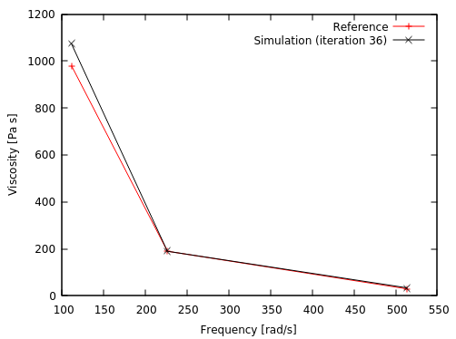
Figure 2: viscosity of the viscoelastic material as a function of the rheometer’s frequency (reference and simulation).
The viscosity is defined as  ,
where
,
where  is the maximum tangential stress and
 is the maximum strain. As can be seen
in Figure 3, requires some time before reaching
a steady-state value. In order to calculate properly the viscosity,
it is necessary to set the number of periods to a value which is
high enough to allow the reaching of the steady-state (in this case 70
seems to be enough). The template only averages the viscosities obtained
from the second half of the force history plot in Figure 3.
is the maximum strain. As can be seen
in Figure 3, requires some time before reaching
a steady-state value. In order to calculate properly the viscosity,
it is necessary to set the number of periods to a value which is
high enough to allow the reaching of the steady-state (in this case 70
seems to be enough). The template only averages the viscosities obtained
from the second half of the force history plot in Figure 3.
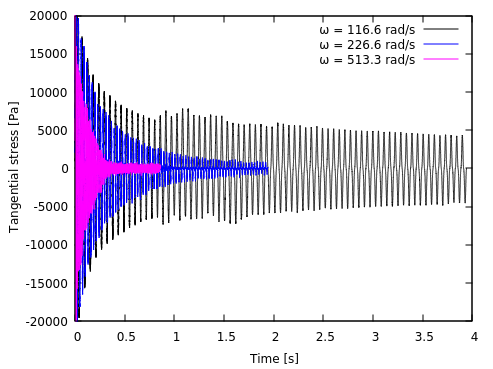
Figure 3: tangential stress as a function of time obtained
at iteration 36. Each iteration consists of 3
simulations performed with the rotation frequencies
,
and . The number of
periods that are simulated is equal to 70 to allow
the reaching of a steady-state.