Soil calibration

Description

This text describes how to perform a cohesive soil calibration using the soilCalibration template.

Introduction

A particle bed is generated with an enhanced gravitational acceleration, furnishing realistic initial values for the cohesive stresses. Afterwards the default gravity is restored and an excavation tool is inserted into the particle bed, twisted and rotated. The forces and torques on the tool are calculated and compared with reference values.

This case has seven calibration parameters: the particle Young’s modulus, the particle-particle and particle-tool coefficients of static and rolling friction, and the maximum cohesive stress. The tool Young’s modulus is made equal to the particle Young’s modulus.

Detailed descriptions

Contact model and coarsegraining factor

The contact models used by the soilCalibration template are the normal Hertz, tangential history, rolling friction epsd2 and cohesion adaptive.

The coarsegraining factor is defined in the input file soil_calib.casx under coarsegraining and it is set to 2.

Material properties and particle size distribution

The values of the material properties and the specifications of particle shape, size and distribution are defined in the file soil_calib.casx. In this example we use a polydisperse distribution of spheres.

Calibration case settings

Inside the measurements directory live three files with the reference data for the penetration force as a function of the penetration depth, and for the twisting and excavation torques as functions of the rotation angles. They are the penetrate.CSV, twist.CSV and excavate.CSV, respectively. Here synthetic data is used.

More information about the case settings can be found in the calibration template documentation.

Running the tutorial and analyzing the results

The user can run the tutorial via command line as follows:

aspherix-calibration run -in soil_calib.casx -np 8

where the command-line argument -np 8 is used to set the number of processors used by the DEM simulations to 8. The particle bed generation is always done in serial, to minimize the sensitivity of the results to the number of MPI processes.

Some data output is suppressed by default with the setting dump 0 in the soil_calib.casx script. This can be activated by changing this setting to dump 1. In this case, a large amount of data will be generated (around 1 TB) and the calibration may crash if there is not enough disk space.

The final calibrated values i.e. those that minimize the quality function are written to the file calibrated_params.txt:

# paramName bestVal qf@bestVal fnEvalfBestVal
Y_p 3e+07 0.333569 44
c_frict_pp 0.433333 0.333569 44
c_frict_pw 0.433333 0.333569 44
c_rollFrict_pp 0.661111 0.333569 44
c_rollFrict_pw 0.7 0.333569 44
maxCohesiveStress_pp 11832.2 0.333569 44

These values are in SI units.

The convergence of the results are attested by analysing the data in the file calibration/results/conv.dat (see below), showing that the quality function qf_total decreases as the number of iterations nIter increases.

# nIter         Y_p       c_frict_pp       c_frict_pw   c_rollFrict_pp   c_rollFrict_pw   maxCohesiveStress_pp         qf_total
 1            3e+07              0.5              0.5             0.65              0.7                11832.2          2.02798
 2      3.66667e+07              0.5              0.5             0.65              0.7                11832.2          1.84723
 4            3e+07         0.566667              0.5             0.65              0.7                11832.2          1.53023
 5            3e+07         0.433333              0.5             0.65              0.7                11832.2          0.49195
17            3e+07         0.433333         0.433333             0.65              0.7                11832.2         0.488792
34            3e+07         0.433333              0.5         0.683333         0.766667                11832.2          0.47733
44            3e+07         0.433333         0.433333         0.661111              0.7                11832.2         0.333569

The python scripts plot_convergence.py and plot_results.py can be used to plot convergence results and the comparison between the calibrated DEM simulation and reference results, respectively: see the figure below.

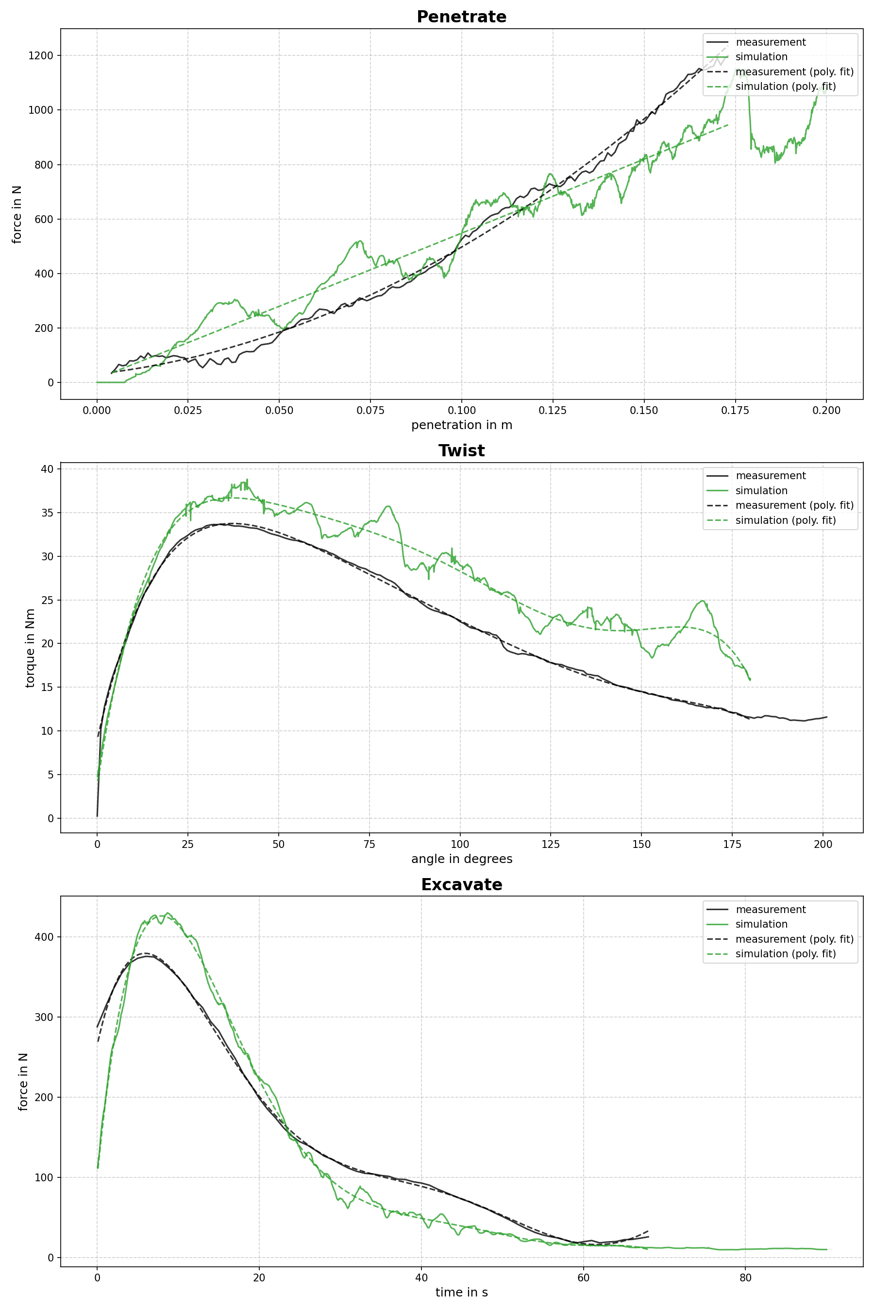
Figure 3: comparison between experimental and calibrated DEM data.

Inside the folder soilCalibration/calibration/workDir/workDir.44/Aspherix/soilCalibration one can find the DEM simulation log files and results, that can e.g. be visualized in ParaView, for the DEM simulation that furnishes the smallest value for the quality function.