Wear model calibration

Note

This example requires a BASH environment. On Windows for instance a “git bash” or similar.

Description

This text describes how to calibrate the combined wear model of Roessler and Katterfeld [1] using the calibration template wear.

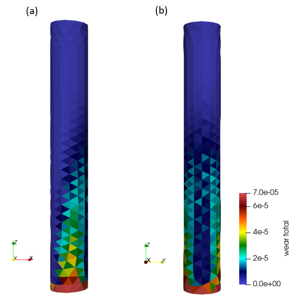
Figure 1: wear on a cylinder: (a) side view, and (b) front view. Simulation run with the calibrated wear model coefficients i.e. k_finnie = 6.59e-13 [m s^2/kg], k_archard = 5.59e-08 [-] and k_deformation = 3.44e-14 [m s^2/kg].

Introduction

In this tutorial, a cylinder is submerged in a particle bed and subsequently subject to surface wear by particle impingement. The three parameters of the combined wear model, i.e. k_finnie, k_archard and k_def, are calibrated by solving an optimization problem that compares DEM simulation results generated with k_finnie = k_archard = k_def = 1.0 against reference data for the wear rate at different pairs of points on the surface of the cylinder. See the mathematical details in the calibration template wear. Here the points are located at the front and sides of the cylinder, and at three different heights, to capture wear resulting from both orthogonal and shear collisions. A total of six pairs of points is used in this example.

To obtain the reference wear rates, experimental measurements of the cylinder diameter over time at the different pair of points is needed. These measurements can be obtained e.g. using a micrometer. The wear rates are calculated from the measured data using the provided script process_exp_data.py, as described in detail in the calibration template documentation. The calibration model is based on the assumption of a linear wear evolution over time, in agreement with literature data [1]. In order to evaluate the accuracy of this assumption for any specific data set, the script process_exp_data.py generates figures displaying the eroded thickness against time: see figure 2 below. If significant deformation of the tool is observed in the experimental setting, it is possible that the linear wear assumption will only be valid at the initial stages of surface wear. In this case, it is recommended that only the data points at this initial stage are used. The model adopted in the wear calibration template does not impose any mesh deformation.

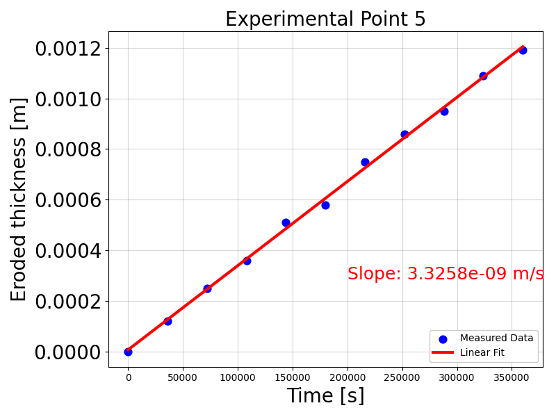
Figure 2: reference eroded thickness and corresponding best-fit line.

Detailed descriptions

Contact model and coarsegraining factor

The contact models used by the wear calibration template are fixed to normal Hertz, tangential history and rolling friction epsd2.

The coarsegraining factor is defined in the input file input.casx under coarsegraining and set to the value 3 by default.

Material properties and particle size distribution

The values of the material properties and the specifications of particle shape, size and distribution are defined in the file input.casx. In this example we use the particle shape multisphere, whose geometry is specified in the file data/multisphere.csv:

-0.77e-3 0 0 2.6e-3
1.65e-3 0 0 1.9e-3

Calibration case settings

The files data/mesh_command_move_bed.asx and data/mesh_command_generate_wear.asx are used to specify (i) the mesh representing the tool subject to wear, and (ii) its location in the simulation domain. Here they are given by

mesh id tool material tool solid yes mesh_modules { sink_mesh } file ../../../../data/cylinder.stl translate ( 0, 0, 0.61111 ) scale_axes ( 1, 1, 0.9 )

and

mesh id tool material tool solid yes mesh_modules { wear } file ../../../../data/cylinder.stl translate ( 0, 0, 0.61111 ) scale_axes ( 1, 1, 0.9 )

respectively. If different mesh geometries are used, one has to replace the cylinder.stl entry by the corresponding file name, and possibly the commands for mesh placement such as translate and scale_axes: the remaining entries of the files data/mesh_command_move_bed.asx and data/mesh_command_generate_wear.asx need to be kept unchanged.

The file measurements/points_coordinates.txt specifies the spatial coordinates of the pairs of points used in the calibration (in meters), i.e. the points where the experimental data was obtained, written in the reference frame of the simulation:

(0.03288891, -0.000131884, 0.317) (-0.03021109, -0.000131884, 0.317)
(0.03288891, -0.000131884, 0.347) (-0.03021109, -0.000131884, 0.347)
(0.03288891, -0.000131884, 0.377) (-0.03021109, -0.000131884, 0.377)
(0.00133891, -0.031681884,0.317 ) (0.00133891, 0.031418116, 0.317)
(0.00133891, -0.031681884, 0.347) (0.00133891, 0.031418116, 0.347)
(0.00133891, -0.031681884, 0.377) (0.00133891, 0.031418116, 0.377)

As mentioned previously, here we use six pairs of points: three at the front and three at the sides of the cylinder, and at three different heights. The calibration template wear page explains how to obtain these coordinates in the reference frame of the simulation.

More information about the case settings can be found in the calibration template wear documentation.

Running the tutorial and analyzing the results

The user can run the tutorial via command line as follows:

aspherix-calibration run -in input.casx -np 4 -skip-qf-check true

where the command-line argument -np 4 is used to set the number of processors used by the DEM simulations to 4. The -skip-qf-check true is necessary because the quality function is evaluated by a python script.

The calibrated wear coefficients are written to the file calibration/results/calibrated_wear_coefficients.txt, together with the global relative error. The results are displayed below, and show a relative error of 3.12%.

k_deformation: 3.440428789680292e-14
k_finnie: 6.590637184325819e-13
k_archard: 5.593433600874002e-08
Relative error: 3.12%

These values are in SI units i.e. k_deformation in [m s^2/kg], k _finnie in [m s^2/kg] and k_archard and Relative error are non-dimensional. The error metric use all pairs of points, and the level of agreement varies for each pair. This can be accessed in the file calibration/simulations/Aspherix/test1/logInit.txt, that lists both experimental and DEM wear rates, in [m/s], for each pair of points:

DEM total wear rates at calibrated points = [3.5e-10 4.0e-10 5.9e-10 5.8e-09 3.9e-09 2.8e-09]
EXP wear rates at calibrated points =       [3.3e-10 4.1e-10 6.2e-10 6.1e-09 3.9e-09 2.8e-09]

The calibration automatically generates the figure in calibration_comparison.png, inside the folder calibration/simulations/Aspherix/test1, showing comparisons between the experimental and calibrated DEM data: see Figure 3 below.

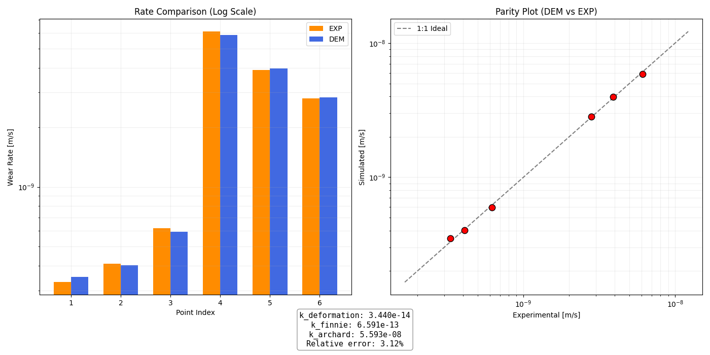
Figure 3: comparison between experimental and calibrated DEM data.

Inside the folder calibration/simulations/Aspherix/test1 one can find the file ke_versus_time.txt (ke stands for the kinetic energy of the particle system), that is useful for analysing if a statistical steady state has been reached before the activation of the wear model. Additionally, several figures can be found in this folder, such as figure 4 below. They display the time evolution of the eroded thickness for each pair of points, obtained from the DEM simulations with k_finnie = k_archard = k_def = 1.0. They are useful for checking if the assumption of linear wear is satisfied in the simulation.

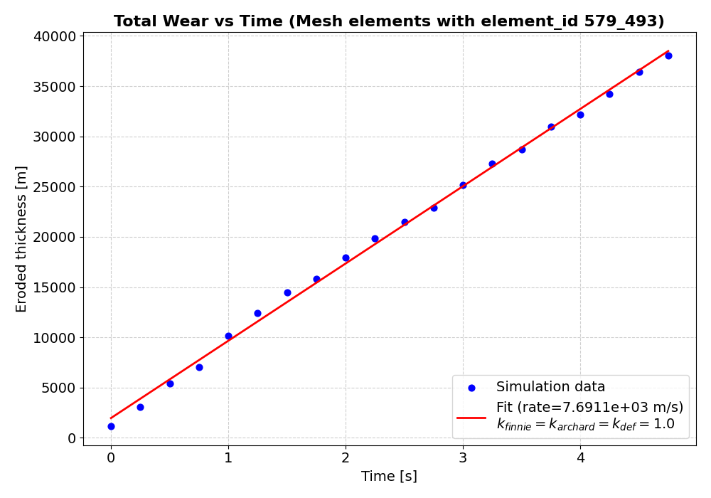
Figure 4: eroded thickness and corresponding best-fit line obtained form the DEM simulation with k_finnie = k_archard = k_def = 1.0.

Also inside the calibration/simulations/Aspherix/test1 the file logInit.txt contains useful information about the DEM simulations. For example, if any warnings are issued they will be displayed in this file. One should verify that the there is no warnings about the time step beeing too large.

The mesh triangles that are used in the calibration, i.e. those whose location are closest to the coordinates specified in points_coordinates.txt, can be visualized interactively by opening the generated file calibration/simulations/Aspherix/test1/wear_extraction_verification.html using a web browser. For example, using the terminal command firefox wear_extraction_verification.html. A snapshot is shown in Figure 5 below. This is useful for checking that the triangle positions correspond to the experimental measurement point locations. In the same folder, the file mesh_triangle_ids.txt contains the ids of the mesh elements used in the calibration. One can verify once again, by inspecting the ‘element_id’ in ParaView, that the triangle locations are correct.

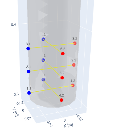
Figure 5: pairs of points used in the wear calibration.

Literature

[1] Roessler, T. and Katterfeld, A. Calibrated and Validated Wear Prediction for Bulk Material Handling Equipment using DEM Simulations. ICBMH2023 - The 14th International Conference on Bulk Materials Storage, Handling and Transportation 11-13th July, 2023, Wollongong, New South Wales, Australia.