wear

Template Info

Target Parameters: k_deformation, k_finnie, k_archard
Contact Models: normal hertz, tangential history, rolling_friction epsd2
Particle Shapes: sphere, multisphere

This template is used for the calibration of the three coefficients of the combined wear model. The section Template parameters lists the necessary parameters and files that have to be specified to use this template. A tutorial illustrating the use this template can be found in this other page. The Python virtual enviroment (e.g. python3-venv, but not python3-virtualenv) needs to be installed in one’s machine in order to run this calibration template.

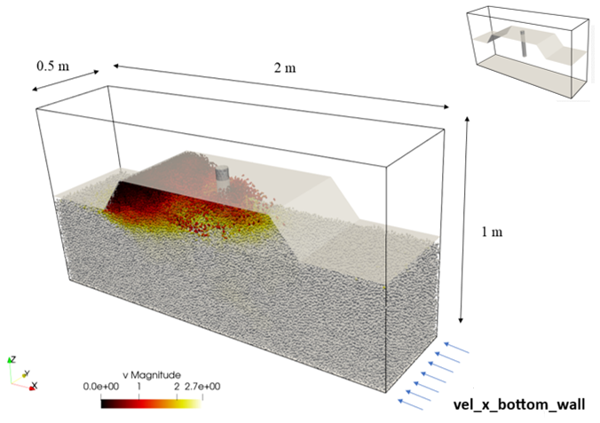
_images/fig_wear_calibration_2.png — Figure 1: Simulation result obtained from `wear` calibration template.

Simulation phases

Initialization

In the initialization phase a particle bed is generated inside a domain with periodic boundary conditions on y and x directions, and a constant velocity is imposed at the bottom plate on the negative x direction (see figure 1). This is done by two subsequent DEM simulations: (i) init and (ii) move-bed.

The tool that will be subject to particle wear is introduced in the move-bed simulation, and the simulation time is controlled by the move_bed_time parameter. The tool, which is a cylinder in the example depicted in figure 1, is submerged in the particle bed with a speed of 0.05 [m/s] in the negative z direction and therefore the move_bed_time has an influence on its final location. If move_bed_time is too large, the tool can move outside of the domain. This will abort the simulation and output an error message. The initial position of the tool is also important. Its point with the lowest z coordinate has to be above the top of the particle bed at the moment of the tool insertion. Otherwise particles can get stuck on the tool surface, leading to unrealistic results. The initial and final placements of the tool in the domain can be checked a posteriori e.g. in ParaView: vtk files are written to calibration/simulations/Aspherix/test1/post. For quick results, an initial calibration with a large coarsegraining factor can be done.

The stl file representing the tool geometry is specified with the Aspherix Solver mesh command. The position of the tool inside the simulation domain can be adjusted using the different keywords of the mesh command, such as translate, rotate and scale. This should be specified in the file data/mesh_command_move_bed.asx. The command should always start with mesh id tool material tool solid yes mesh_modules { sink_mesh }.

Optimization

This calibration template uses the mesh module wear and therefore the wear is a passive scalar that does not have an influence on the particles motion, since no actual deformation is applied to the mesh. Thus, a single DEM simulation is executed in the optimization phase, and the results of this simulation are used in the framework described below for the calibration of the three wear coefficients. In this phase, the wear is calculated using k_finnie = k_deformation = k_archard = 1.0, for reasons explained in section Quality Function below.

Quality Function

The calibration framework is based on the assumption that the wear evolves linearly with time:

$W_{\text{thickness, exp}} = A_{\text{exp}} t \quad \therefore \quad \frac{\partial W_{\text{thickness, exp}}}{\partial t} = A_{\text{exp}} = \text{const}$

which has been experimentally verified e.g. in Roessler and Katterfeld [1]. We provide a tool for post-processing experimental data that can be used to validate this assumption (see the Measurement file section). For performance, we do the calibration for the wear rate instead of the wear itself because, under the assumption of linear wear, the wear rate is independent of time. This allows us to use DEM simulation times , set by the simulate_wear_time in the calibration input script, that are much smaller than the actual time that the tool will be subject to wear in the experimental apparatus. After the calibration is finalized, a time-stretching approach can be used to extrapolate results to longer times, as described in the section Time stretching below.

At a given instant of time the wear (height) that has been accumulated in a mesh triangle is given by

$W_{\text{height, DEM}} = k_{\text{finnie}} \sum_{\gamma > 1.0^{\circ}} \frac{0.5 m_p v_p^2 f(\gamma)}{S_{\text{tri}}} + k_{\text{def}} \sum_{\text{all } \gamma} \frac{0.5 m_p v_n^2}{S_{\text{tri}}} + k_{\text{archard}} \sum_{\gamma \leq 1.0^{\circ}} \frac{W L}{S_{\text{tri}} H}.$

The notation that is used here is the same as in the mesh module wear documentation, the summation is for all particle-wall collisions, and the combined wear model of Roessler and Katterfeld [1] is adopted.The eroded thickness i.e., the decrease over time of the distance between two points on the tool surface, is obtained by summing the wear height of the two corresponding mesh elements. The resulting eroded tickness rate can be written in a compact way after introducing the following definitions:

$A_{\text{finnie}} := \frac{\partial}{\partial t} \sum_{\substack{\gamma > 1.0^{\circ} \\ \text{tri 1 and tri 2}}} \frac{0.5 m_p v_p^2 f(\gamma)}{S_{\text{tri}}},$

$A_{\text{def}} := \frac{\partial}{\partial t} \sum_{\substack{\text{all } \gamma \\ \text{tri 1 and tri 2}}} \frac{0.5 m_p v_n^2}{S_{\text{tri}}},$

$A_{\text{archard}} := \frac{\partial}{\partial t} \sum_{\substack{\gamma \leq 1.0^{\circ} \\ \text{tri 1 and tri 2}}} \frac{W L}{S_{\text{tri}} H}.$

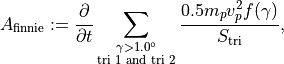
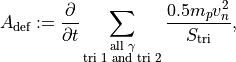
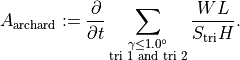
where tri 1 and tri 2 stands for the sum for the two mesh triangles. The eroded thickness rate is then

$\frac {\partial}{\partial t} W_{\text{thickness, DEM}} = k_{\text{finnie}} A_{\text{finnie}} + k_{\text{def}} A_{\text{def}} + k_{\text{archard}} A_{\text{archard}}.$

Imposing equality of the experimental and simulated eroded thickness rates, we arrive at the expression defining the optimization problem:

$k_{\text{finnie}} A_{\text{finnie}} + k_{\text{def}} A_{\text{def}} + k_{\text{archard}} A_{\text{archard}} = A_{\text{exp}}$

where the $A_{\text{exp}}$ [m/s] is provided by the user (see the details in section Measurement file), $A_{\text{finnie}}$ [m/s], $A_{\text{def}}$ [m/s] and $A_{\text{archard}}$ [m/s] are obtained from the DEM simulation i.e. the optimization phase with k_finnie = k_deformation = k_archard = 1.0 described above, and the calibrated wear coefficients $k_{\text{finnie}}$ , $k_{\text{def}}$ and $k_{\text{archard}}$ are calculated by the optimizer. If more than one pair of points is used for the calibration, the equation above is written using matrix notation, where the $A_{\text{finnie}}$ [m/s], $A_{\text{def}}$ [m/s] and so on are vectors whose components correspond to each pair of points. The optimizer uses a constrained weighted least squares optimization based on the SciPy solver scipy.optimize.lsq_linear.

The spatial coordinates of the pairs of mesh elements used in the calibration, in the reference frame of the DEM simulation, have to be specified in the file measurements/points_coordinates.txt. The example below corresponds to a case where the tool is a cylinder of radius equal to 0.1 [m], whose axis is aligned with the z axis and the center of its lower circle is at the origin of the reference frame of the DEM simulation:

(-0.1, 0.0, 0.05) (0.1, 0.0, 0.05)
(-0.1, 0.0, 0.15) (0.1, 0.0, 0.15)
(-0.1, 0.0, 0.25) (0.1, 0.0, 0.25)

In this example, three pairs of points are specified, at z = 0.05 [m], 0.15 [m] and 0.25 [m]. The experimentalist would have to measure the diameter of this cylinder for different time instants, at these z locations, to determine the time evolution of the eroded thickness i.e. how much the diameter decreases over time due to the particle wear.

After specifying the tool location inside the simulation domain, in the files data/mesh_command_move_bed.asx and data/mesh_command_generate_wear.asx, the user can obtain the coordinates of a single point on the tool surface in the reference frame of the DEM simulation by (i) running the calibration with estimated point coordinates until the move-bed initialization phase is completed, with a larger coarsegraining factor for quick results, (ii) visualizing the resulting vtk files, using e.g. ParaView, that are stored in calibration/simulations/Aspherix/test1/post. The remaining point coordinates in the reference frame of the DEM simulation can be obtained with pen and paper using geometrical considerations or directly in ParaView.

When the input parameter averaging_radius is larger than zero, the wear in each mesh triangle used in the calibration is the averaged wear of the neighboring triangles, within a distance of averaging_radius [m] from the main triangle. This can improve results by reducing the noise of the wear data that results e.g. when the resolution of the mesh is very fine, with mesh triangles of the same size (or smaller) than the particle size.

Measurement file

The values of the experimental eroded thickness rates, in [m/s], have to be specified in the file measurements/experimental_wear_rates.txt. The format is illustrated in the example below

0e-10
1e-10
8e-10

where the value in each line correspond to a different pair of points e.g. at z = 0.05 [m], 0.15 [m] and 0.25 [m] in the cylinder example of the previous section. If one has thickness measurements over time, obtained e.g. with a Caliper or Micrometer, one can use the provided python script process_exp_data.py to read this measurements and generate the experimental_wear_rates.txt file before running the calibration. The measured values have to be written in a spreadsheet named wear_exp.xlsx where the first column has the time values in hours and the remaining columns have the thickness measurements in millimeters, for each pair of points. The script process_exp_data.py uses the Python libraries pandas, openpyxl and matplotlib, that need to be installed before running the script.

Time stretching

Time stretching can be used to obtain e.g. the wear after 10 hours of operation by running a much shorter simulation of e.g. 10 seconds. This is based on the assumption that the wear increases linearly over time, and is a scaling that is applied to the wear coefficients k_deformation, k_finnie and k_archard after the calibration is finalized. The procedure is illustrated in the equations below for this case where 10 hours of operation is simulated by a 10 seconds simulation, and can be easily adapted to other scenarios.

By applying this scaling to the calibrated wear coefficients, the wear that is visualized e.g. in ParaView after 10 seconds of simulation should be interpreted as the wear after 10 hours of operation.

Template parameters

The following files have to be provided in order to use this calibration template

input.casx
data/mesh_command_move_bed.asx
data/mesh_command_generate_wear.asx
data/multisphere.csv
data/my_mesh.stl
measurements/points_coordinates.txt
measurements/experimental_wear_rates.txt
measurements/dummy.txt

where data/multisphere.csv is only needed if multisphere particles are used and data/my_mesh.stl can of course have a different name.

Additionally, the parameters below have to be provided in the input.casx calibration script, either as variable or param_fixed:

Parameter name	Parameter Description	Typical value
coarsegraining	particle coarsegraining factor	3 [-]
rho_p	particle density	2500.0 [kg/m^3]
rho_w	wall density	2500.0 [kg/m^3]
rho_tool	tool density	6000.0 [kg/m^3]
Y_p	particle Young’s modulus	4.5e+06 [Pa]
Y_w	wall Young’s modulus	0.9e+07 [Pa]
Y_tool	tool Young’s modulus	0.9e+07 [Pa]
poissonsR_p	particle Poisson’s ratio	0.35 [-]
poissonsR_w	wall Poisson’s ratio	0.35 [-]
poissonsR_tool	tool Poisson’s ratio	0.35 [-]
c_rest_pp	particle-particle coefficient of restitution	0.8 [-]
c_rest_pw	particle-wall and particle-tool coefficient of restitution	0.4 [-]
c_frict_pp	particle-particle coefficient of friction	0.6 [-]
c_frict_pw	particle-wall and particle-tool coefficient of friction	0.5 [-]
c_rollFrict_pp	particle-particle coefficient of rolling friction	0.06 [-]
c_rollFrict_pw	particle-wall and particle-tool coefficient of rolling friction	0.18 [-]
hardness_w	material hardness used by the Archard component of the wear model	1.2e+05 [Pa]
dt_DEM	DEM time step	0.7e-4 [s]
dt_output_wear	output time step	0.25 [s]
simulate_wear_time	simulation time of the generate-wear phase	5.0 [s]
move_bed_time	simulation time of the move-bed phase. This has an influence on the final position of the tool inside the particle bed.	4.86 [s]
vel_x_bottom_wall	x component of the bottom wall velocity vector	-3.0 [m/s]
averaging_radius	radius of neighbor mesh-triangle wear-smoothing	0.01 [m]

Restrictions

If the specified coarsegraining is excessively large, and the resolution of the stl mesh representing the tool is very fine, the DEM simulations used in the calibration might abort with a neighborlist overflow error. In that case, possible solutions are (i) use a smaller coarsegraining factor, and (ii) use a coarser mesh.

References

[1] Roessler, T. and Katterfeld, A. Calibrated and Validated Wear Prediction for Bulk Material Handling Equipment using DEM Simulations. ICBMH2023 - The 14th International Conference on Bulk Materials Storage, Handling and Transportation 11-13th July, 2023, Wollongong, New South Wales, Australia.