 Home
HomeradiationModel: P1CFDEM
The P1CFDEM model introduces a radiation field G into the solver that is solved alonside the fluid flow fields.
Syntax
Configured in radiationProperties dictionary:
radiationModel   P1CFDEM; // select the P1CDFEM radiation model

radiation        <bool>;
solverFreq       <integer>;
radiation= switch radiation modeling on/offsolverFreq= number of CFD timesteps per radiation solution
Additionally the radiation model requires that models for the absorption-emission, the scattering and the soot be defined:
absorptionEmissionModel <word>;

scatterModel            <word>;

sootModel               <word>;
absorptionEmissionModel= the absorption-emission model (see absorptionEmissionCFDEM)scatterModel= the scattering model (see constantScatterCFDEM)sootModel= the soot model (for default behaviour:none)
Note
The abovementioned absorption-emission and scattering models add an additional <modelName>Coeffs sub-dicitonary for configuration.
Additional Settings
In addition to configuring the P1CFDEM model in constant/radiationProperties it is necessary to add an appropriate settings for solving for the radiation field G.
This requires setting the boundary conditions for G.
The boundary conditions for G are found in the starting time directory for the CFDEM case.
For example in 0/G under boundaryField we set Marshak-radiation boundary conditions for the walls:
wall
{
    type            MarshakRadiation;
    T               T;
    emissivityMode  lookup;
    emissivity      uniform <value>;
    value           uniform 0; // (initial condition for compatibility, overwritten by the BC)
}
This boundary condition calucates the (radiative) heat flux at the wall:

with  being the emissivity field at the boundary defined in the
boundary condition:
being the emissivity field at the boundary defined in the
boundary condition:
Note
For more details regarding all the available boundary conditions please consult you OpenFOAM distributions documentation.
The the solver for G is configuring in system/fvSolution and system/fvSchemes.
For example in system/fvSolution under solvers:
solvers
{
    "(G|GFinal)"
    {
        solver          PCG;
        preconditioner  DIC;
        tolerance       1e-06;
        relTol          0.1;
    }
}
For example in system/fvSchemes under laplacianSchemes:
laplacianSchemes
{
    laplacian(gammaRad,G) Gauss harmonic corrected;
}
Note
For more details regarding all the available finite-volume solvers and schemes please consult you OpenFOAM distributions documentation.
Examples
radiationModel   P1CFDEM;

radiation        true;
solverFreq       10;   // every 10 CFD timesteps

absorptionEmissionModel absorptionEmissionCFDEM;

scatterModel            constantScatterCFDEM;

sootModel               none;
absorptionEmissionModel= the absorption-emission model (see absorptionEmissionCFDEM)scatterModel= the scattering model (see constantScatterCFDEM)sootModel= the soot model (for default behaviour:none)
Note
For details regarding the configuration of the absorption-emission model and the scatter model please refer to their documentation.
Description
In order to activate the radiation model the file constant/radiationProperties
must be present in the CFD case directory. Otherwise radiation will not be taken into
account.
Boundary conditions and initial field values for the radiation intensity G must
be defined in 0/G.
The P1 model solves a diffusion equation for incident radiation. The model is limited
to applications with optical thickness  . The equation being solved is:

with the diffusion coefficient  :
:
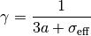
The absorptivity  ,
,  and emission contribution
  come from the
absorption model. The effective scattering coefficient
come from the
absorption model. The effective scattering coefficient  comes
from the scattering model. The Stefan-Boltzmann constant
comes
from the scattering model. The Stefan-Boltzmann constant

The energy source term is calculated as Sh() = (Ru() - Rp() * T^4) with
Ru() = a * G - 4E) and Rp() = 4*e*sigmaSB leading to
Sh() = a * G - 4*(e*sigmaSB * T^4 + E)
The temperature source term is calculated as: ST() = Sh()/(rho * Cp)
For further discussion of the model, consult [1].
Literature
[1] J. Mačak, C. Goniva, St. Radl (2023). “Predictions of the P1 approximation for radiative heat transfer in heterogeneous granular media” Particuology 82: 25-47
Restrictions
Optically thin media.