 Home
HomeTheory of CFD-DEM
Introduction into CFD-DEM
The combination of Computational Fluid Dynamics (CFD) and Discrete Element Methods (DEM) is a mixed Eulerian-Lagrangian approach initially proposed by Tsuji et al. (1993). This approach models the fluid phase with CFD where the volume averaged Navier-Stokes equations are solved to obtain the velocity and pressure fields. Additionally, the particulate phase is modelled using DEM, a Lagrange method explicitly tracking particle positions and velocities.
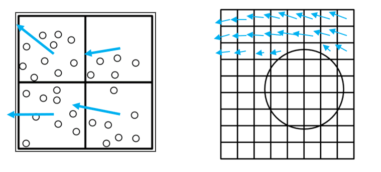
Figure 1: Particle and CFD cell size in unresolved (left) and resolved (right) CFD-DEM setups. The blue arrows in addition indicate the cell-based fluid velocity.
In addition to the interaction forces between solid (particle) phase and liquid phase the spatial scales of the methods to be coupled must be taken into account. The finite volume method commonly applied in CFD solves the governing equations based on discrete volumes (cells), DEM performs its calculations directly for the individual particles. In general, there are two methods in CFD-DEM to connect these two distinct scales: resolved and unresolved CFD-DEM. In resolved CFD-DEM the CFD cells are significantly smaller than the particles, compare Figure 1. With this method fluid flow around the particles is described much more accurately than with the unresolved approach. However, the resolved CFD-DEM approach requires a large number of CFD cells. As a rule of thumb, a (spherical) particle must be resolved by at least 10 CFD cells along its diameter in every coordinate direction leading to at least 1000 CFD cells per particle. Hence, the required number of CFD cells increases rapidly with the number of particles. Consequently, simulations of only a limited number of particles – up to a few thousand – can be conducted in a reasonable amount of time. In unresolved CFD-DEM the CFD cells are much larger than the particles (Figure 1). This method unlocks the simulation of large problems with millions of particles. Fluid flow, however, is solved with this method on a scale that is much larger than the individual particles and information about the flow around these particles is lost. The fluid velocity is averaged in the CFD cell and the fluid forces are evenly distributed to the particles located in a cell. To complete this approach, force models are required to compute the interaction forces between particles and fluid. With this approach, the computational effort is concentrated on the DEM side for large particle counts.
Note
For unresolved CFD-DEM it is mandatory that the particles are smaller than the CFD cells and that the voidfraction (the ratio of cell volume not occupied by particles to cell volume occupied by particles) does not become too small. Please refer to the documentation of the voidfraction models centre and divided. Moreover, consider using a smoothingModel if your particles are larger than your CFD cells.
- [1] Y. Tsuji, T. Kawaguchi, T. Tanaka,
Discrete particle simulation of two-dimensional fluidized bed, Powder Technology 77(1), 1993
Regimes of fluid-particle interactions
From a modelling perspective different regimes for the interaction of particles and fluid arise. These regimes depend on the density of particles or, more specifically, the particle volume fraction as indicator on how important certain interactions are. Figure 2 illustrates these regimes.
One-Way coupling:
Fluid affects the particle motion
Particles have no impact on the fluid
Only valid for very dilute particle concentrations
Two-Way coupling
Particle motion affects the fluid, e.g. wakes behind particles
Three-Way coupling
Disturbed fluid motion affects further particles
Particles are affected by the wakes of the particles in front of them
Four-Way coupling
Particle-particle interaction, for instance due to collisions
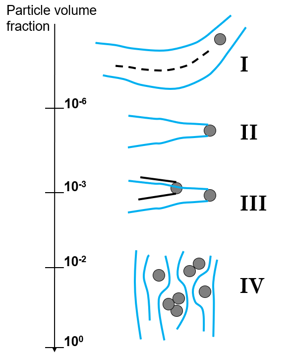
Figure 2: Different regimes of fluid-particle interactions with approximate range of validity for the particle volume fraction.
Drag computation in CFDEMcoupling
Drag laws in CFDEMcoupling are always written in the form
(1)
where  is the drag coefficient,
  the particle cross
section,
the particle cross
section,  the voidfraction, and
  is a
correction function for collective particle effects.
Thus, a drag law is always derived from the drag for a single sphere corrected by
a correction function. The drag coefficient of a single sphere
according to different drag correlations and experiments is depicted in Figure 3.
is a
correction function for collective particle effects.
Thus, a drag law is always derived from the drag for a single sphere corrected by
a correction function. The drag coefficient of a single sphere
according to different drag correlations and experiments is depicted in Figure 3.
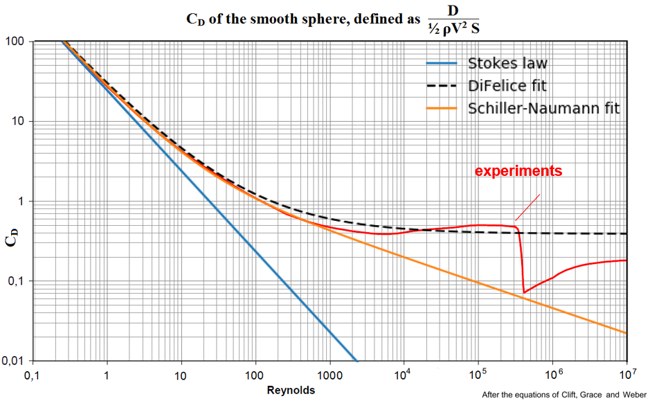
Figure 3: Drag coefficient of a single sphere
according to different drag correlations and experiments.
A typical example for the described approach is the DiFelice drag law where the correlation for the drag coefficient and the correction function are
(2)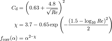
and the correction function depends on the voidfraction and the Reynolds
number as shown in Figure 4.
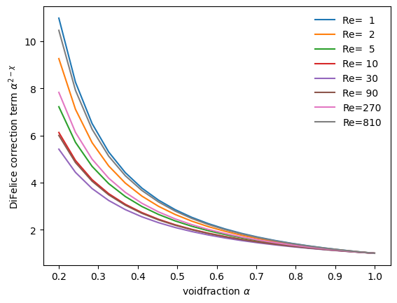
Figure 4: Drag correction function  as used in the DiFelice drag model.
Putting these pieces together leads to the overall behavior shown in Figure 5, where the drag force for different drag laws and an voidfractions is shown. As a general trend, the drag force increases for denser particle packings as the fluid velocity in constricted cross sections increases.
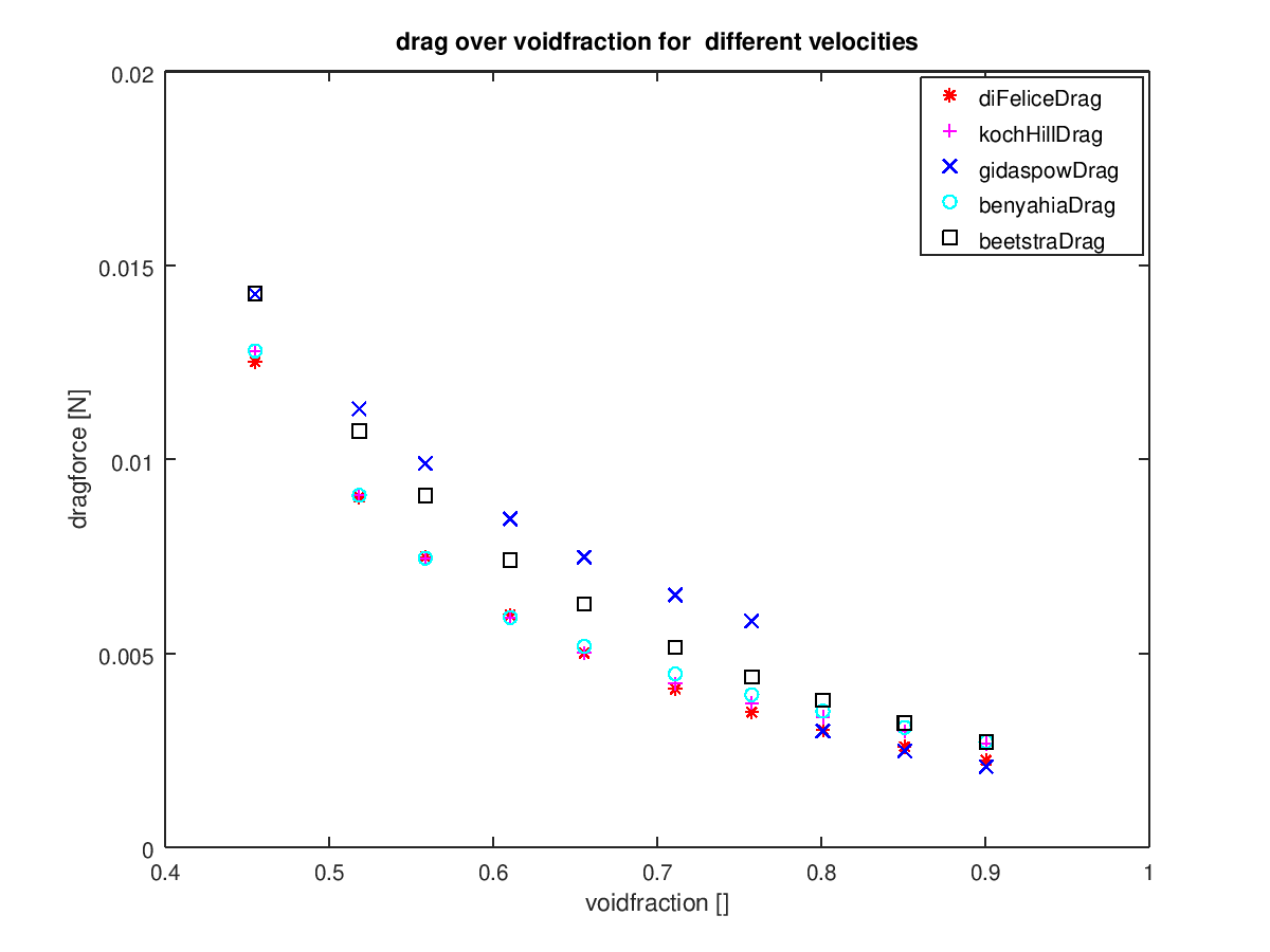
Figure 5: Drag force depending on voidfraction for different drag models in CFDEMcoupling.
In case implicit drag force treatment on the DEM side – as discussed below – is chosen, the drag coefficient for implicit drag handling (see (3)) is computed from the drag force (see (1)) as
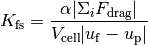
by the drag model and communicated to the DEM accordingly.
Handling of drag force in DEM simulation
On the DEM side the drag force can be accounted for in two ways.
The straightforward way is to directly apply the force calculated by the drag law. This means that the force is constant over one coupling interval, i.e. the number of DEM time steps until the next data exchange. As the particle is accelerated with a constant rate (i.e. a constant force), its velocity is not bounded and can surpass the fluid velocity. This behavior can, for instance, be observed for very long coupling intervals and large drag forces and quickly leads to a diverging simulation.
Implicit handling of the drag force improves on the shortcomings of the explicit
treatment. In this case, the drag force is converted to an expression depending on
a drag coefficient  and the fluid velocity
  :
:
(3)
Instead of just the drag force, the coefficient and the fluid velocity must now be communicated to the DEM and the drag force on the particle is calculated in every DEM time step using (3). Since the drag force is now computed as a value proportional to the relative velocity, the particle velocity is now bounded by the fluid velocity. Overall, this approach is more stable than the explicit treatment discussed above and, therefore, is the default setting in CFDEMcoupling. Figure 6 illustrates the difference between the implicit and the explicit drag force handling on the DEM side.
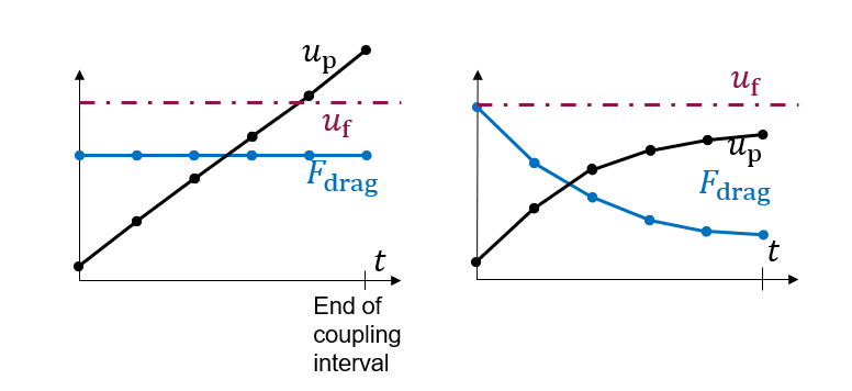
Figure 6: Difference between explicit (left) and implicit (handling) of the drag force on DEM side. With the implicit handling the particle velocity is cannot exceed the fluid velocity.