dividedVoidFraction

Syntax

Defined in couplingProperties dictionary.

voidfractionModel divided;
dividedProps
{
    alphaMin         scalar;
    interpolation    Switch;
    volScale         scalarList;
    volScaleGlobal   scalar;
    porosity         scalar;
    procBoundaryCorrection Switch;
    verbose          Switch;
    resolution       vector;
}

alphaMin = minimum limit for voidfraction (default: 0.3)
interpolation = flag to interpolate voidfraction to particle positions (default: false)
volScale = scaling (per type) of the particle volume to account for porosity or agglomerations. (default: 1 for each particle type)
volScaleGlobal = volScale factor to apply for all particle types. This conveniently sets all elements of the volScale list to the same value. (default: 1)
porosity = diameter of the particle’s representation is artificially increased according to porosity * Vparticle. In contrast to volScale, however, the volume remains unaltered. (default: 1)
procBoundaryCorrection = allow for correction at processor boundaries. This requires the use of engineIB and vice versa. (default: false)
verbose = flag for debugging output (default: false)
resolution = resolution for superquadric particles. The resolution in each coordinate direction specifies the number of points inserted along the particle’s principal half axis in addition to the particle center point. (default: (1 1 1), (3 3 3) for convex particles)

Note

The resolution keyword is only valid for superquadric and convex particles. In contrast to the procedure described below for spheres, the particle volume is not split up into sub-volumes arranged in sphere shells but into a three-dimensional grid in the particle’s principal axes. Points located outside of the particle are not used. Hence, the number of subvolumes used depends also on the particle shape.

The resolution keyword exploits the symmetry of superquadric particles and sets the resolution only in a single octant.

For convex particles, the full resolution of the particle is defined by this keyword, not the resulution per octant. For convex particles the default changes to (3 3 3).
baseDirectory = base directory for search of surface files (default: “.”)

Note

The baseDirectory keyword is only valid for convex particles.
particleSurfaces = list of surface files defining convex bodies. The full file path will be generated using the baseDirectory setting.

Note

The particleSurfaces keyword is only valid for convex particles.

The order of files must be identical to the order of particle_template command definitions on the DEM side.
surfaceCenterPoints = list of center points. If set deactivates the automatic calculation

Note

The surfaceCenterPoints keyword is only valid for convex particles.

Must be in the same order as the list defining particleSurfaces.

Examples

voidfractionModel divided;
dividedProps
{
    alphaMin 0.2;
    volScale ( 1. );
}

particleShapeType "superquadric";
voidfractionModel divided;
dividedProps
{
    alphaMin 0.2;
    resolution (1 1 2)
}

Description

The divided voidFraction model is supposed to be used when a particle (or its representation) is in the size range of a CFD cell. This model splits each particle into a number of sub-volumes and accounts for these sub-volumes individually, hence, distributing the particle volume over neighboring cells if the particle is in the size range of a CFD cell or if it’s center is close to the CFD cell boundary and the particle extends into the neighboring cell.

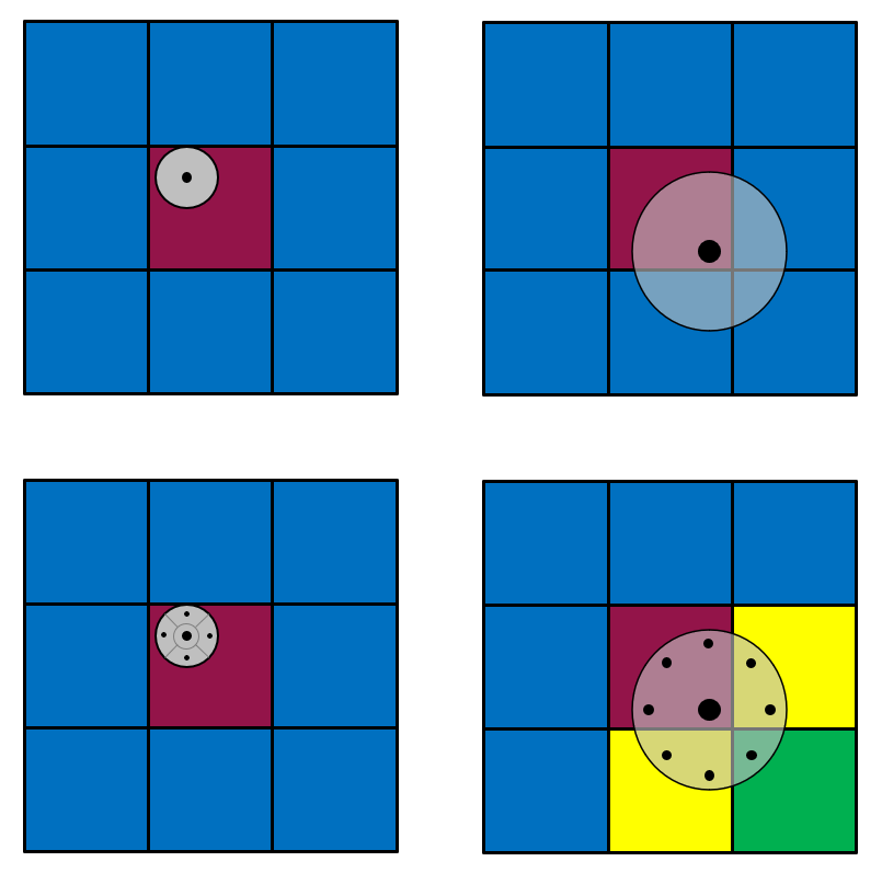
_images/voidfraction_center_divided.png — Figure 1: Comparison of center (top) and divided (bottom) voidfraction model. In contrast to the center model, the divided model accounts for particle volume also in neighboring CFD cells.

The particle (of radius $R$ ) is divided into 29 non-overlapping regions of equal volume. The centroids of these volumes are then used to reproduce each volume. The first volume is a sphere with the center coinciding with the particle center. The radius of the innermost subsphere can then be found as follows:

$\frac{V(r_1)}{V(R)} = \frac{r_1^3}{R^3} = \frac{1}{29} \longrightarrow r_1 = R \left( \frac{1}{29} \right)^\frac{1}{3}$

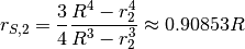
The rest volume is a spherical layer that is divided into 2 layers of equal volume. Position of the border between these two spherical layers in radial direction can be easily obtained:

$\frac{V(r_2)}{V(R)} = \frac{r_2^3}{R^3} = \frac{15}{29} \longrightarrow r_2 = R \left( \frac{15}{29} \right)^\frac{1}{3}$

Each of these spherical layers is later divided into 14 elements of equal volume. Position of the centroid point in radial direction of each volume in the first spherical layer is as follows

$r_{S,1} = \frac{\int r \mathrm{d}V}{\int \mathrm{d}V} = \frac{\int_{\phi_a}^{\phi_b} \int_{\theta_a}^{\theta_b} \int_{r_1}^{r_2} r^3 sin \phi \,\mathrm{d}\phi \,\mathrm{d}\theta \,\mathrm{d}r}{\int_{\phi_a}^{\phi_b} \int_{\theta_a}^{\theta_b} \int_{r_1}^{r_2} r^2 sin \phi \,\mathrm{d}\phi \,\mathrm{d}\theta \,\mathrm{d}r} = \frac{\int_{r_1}^{r_2} r^3 sin \phi \,\mathrm{d}r}{\int_{r_1}^{r_2} r^2 sin \phi \,\mathrm{d}r} = \frac{3}{4} \frac{r_2^4 - r_1^4}{r_2^3 - r_1^3} \approx 0.62761 R$

Similarly, for the second spherical layer (remembering that the external radius is the particle radius):

$r_{S,2} = \frac{3}{4} \frac{R^4 - r_2^4}{R^3 - r_2^3} \approx 0.90853 R$

The region of influence of a particle can be increased artificially by porosity, which blows up the particles, but keeps their volume (for voidfraction calculation) constant.

The particle volume occupied in the CFD domain can be adjusted by the parameter volScale (referred to as $S$ ), using

$V_\mathrm{p} = \frac{4}{3} \pi r^3 S$

In the basic implementation of solvers, the void fraction is calculated based on all particles. Depending on the solver used, the void fraction calculation is also performed for a certain type of particles. The void fraction calculation is based on a three-step approach (reset, set and interpolate), i.e., the void fraction is time interpolated from a previous and a next void fraction field. Custom names for these fields can to be specified in the sub-dictionaries as voidFracFieldNamesPrev and voidFracFieldNamesNext in the couplingProperties dictionary.

If particleShapeType "multisphere" is selected, caluclations are performed for multisphere particles.

Restrictions

None.