Usage of different particle shapes

We first generate a simple case where spherical particles cause wear on a simple chute. Then we clone the basic simulation and use all kinds of nonspherical particles: multispheres, tablets (superquadric particles), fibers and facetted particles (both concave and convex).

This case deomonstrates the simplicity of the usage of different particle shapes, and shows the usage of the tools provided for generating or preparing nonspherical particles.

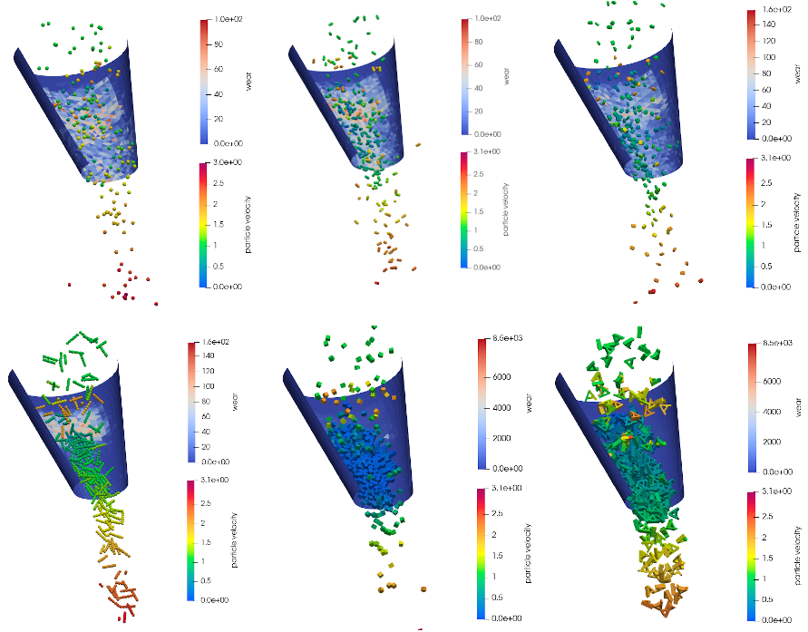
Name of the case: Project_Shapes

Case 1: The spherical base case

As a first step, the particle shape, the used materials command and the simulation domain are defined in the General Settings tab.

General settings

In this simulation we set particles of particle shape sphere:

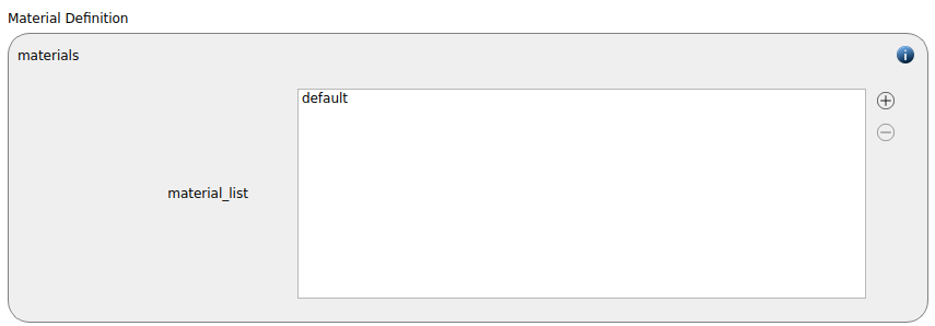
A single material with the name default is used:

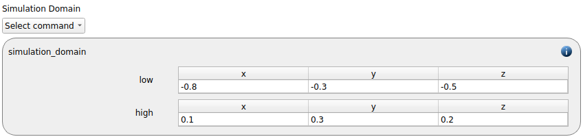
The simulation domain ranging from -0.8 to 0.1 in x, from -0.3 to 0.3 in y and from -0.5 to 0.2 in z direction is created:

Meshes and regions

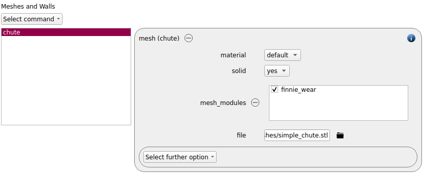
We start by creating a mesh module for calculating the wear on the chute:

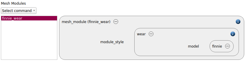
This mesh module is used in the following mesh command command for the chute:

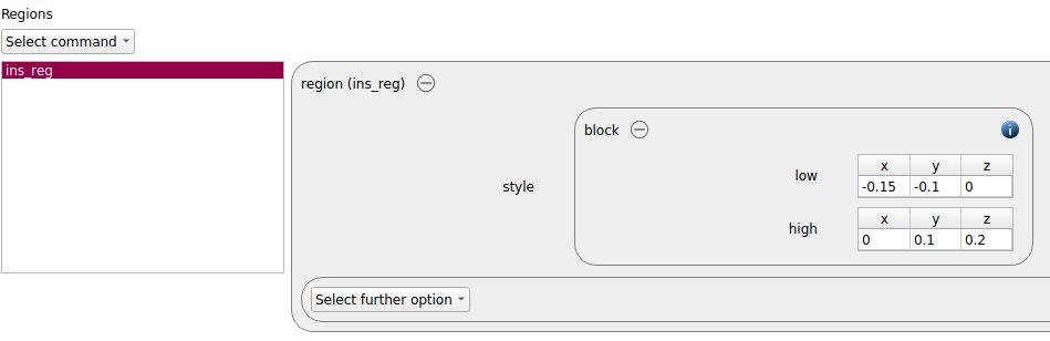
Furthermore, an insertion region command is added in this tab:

Physics models

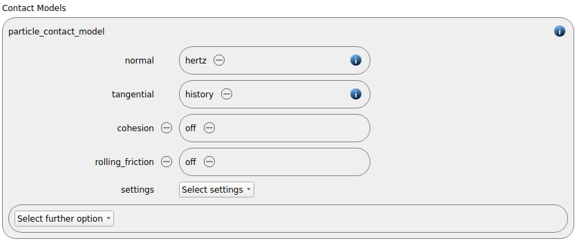
The contact models are now defined. For the particles we use the normal contact model hertz and the tangential model history.

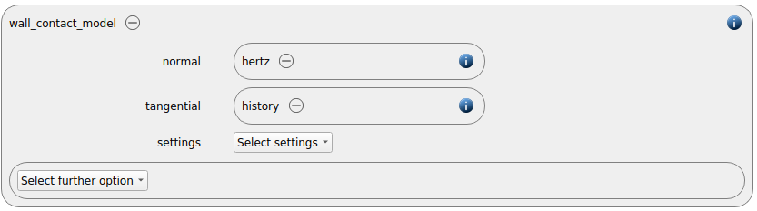
Since we added a mesh in the previous section, a wall contact model is also added automatically to this section. We use the same properties of the particle contact model:

Finally, the gravity is enabled:

Per default the gravity has a magnitude of 9.807 and acts into negative z-direction. These defaults can be changed by either setting the magnitude or the direction manually.

Particles

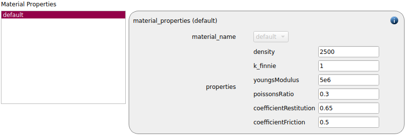
In the general settings tab we only defined a single material type (default), whose settings have to be specified here:

	default
Density	2500
k_finnie	1
Young’s modulus	5e6
Poisson’s ratio	0.3
Coefficient of restitution	0.65
Coefficient of friction	0.5

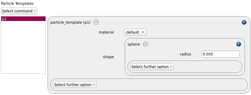
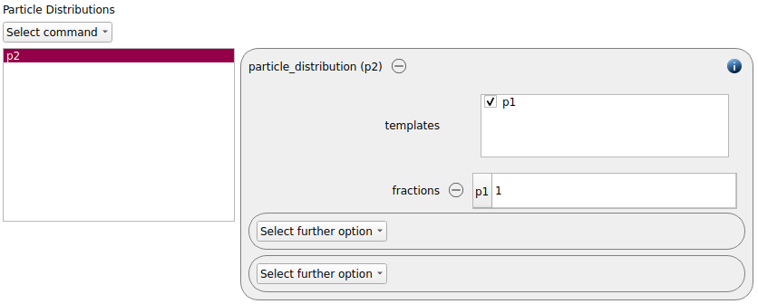
A particle template of shape sphere with radius 0.005 is added and used for a particle distribution:

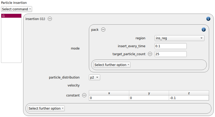
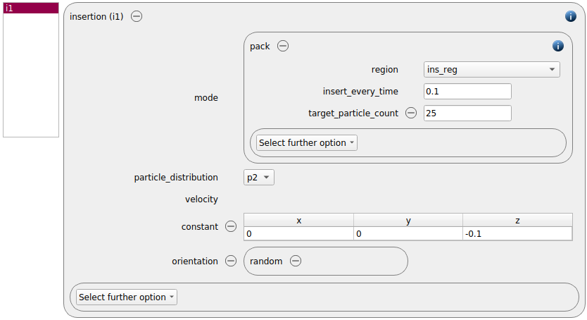
A pack of 25 particles with a velocity of 0.1 m/s in the negative z-direction is now inserted every 0.1 seconds. We use an insertion command command with mode pack:

Simulation control

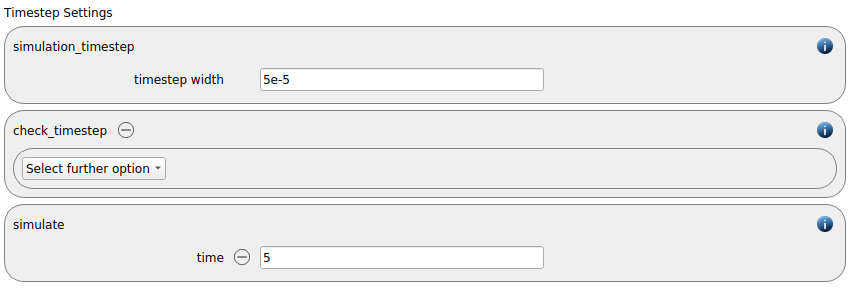
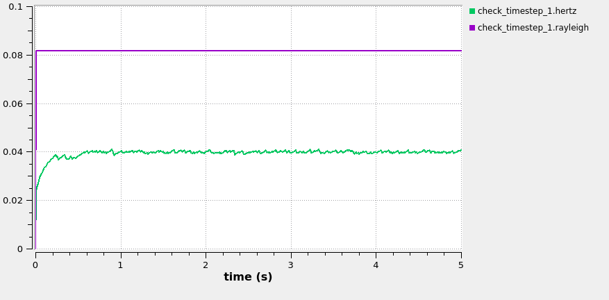
In this tab, we first define the time-step settings such as the desired simulation timestep of 5e-5 seconds and the total simulation time of 5 seconds. Per default also the check_timestep command command is enabled, which throws a warning when the time step exceeds 10 % of the Rayleigh or the Hertz time. These thresholds can be changed by setting an alternative value for hertz_fraction or rayleigh_fraction.

Output settings

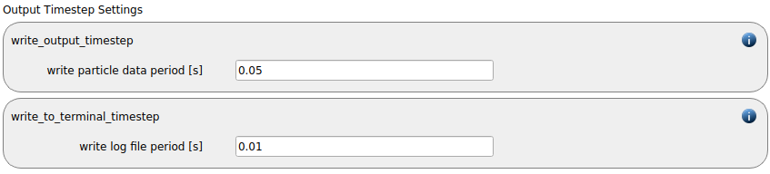
In this tab we first define the timestep width for the file and the terminal output:

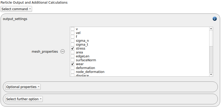
The output_settings command command the takes care that all particle information and the meshes are written to files accordingly. Furthermore it triggers the output of global quantities such as the kinetic energy of the particles or total normal and shear stresses onto meshes to the terminal. Please note that if the output of per-cell information on meshes such as wear, velocity of stress are desired, one has to add the keyword mesh_properties and select the required output.

Running the simulation

After completing the setup and saving it, the simulation can be launched. Change to the Simulation view. First hit the “Check settings” button, and if the check returns “Check settings successfully completed” the simulation can be run by hitting “Start”.

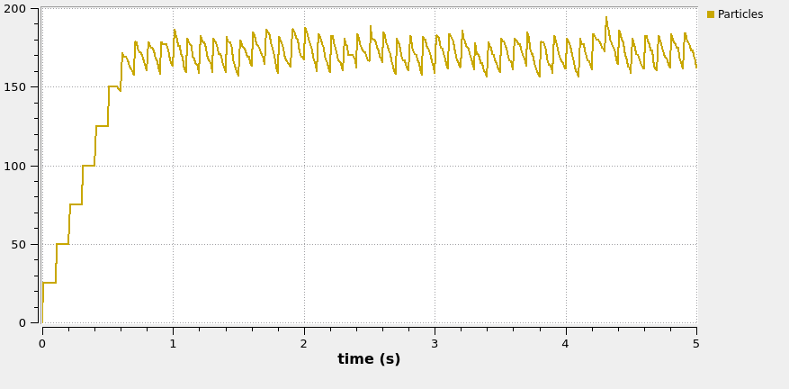
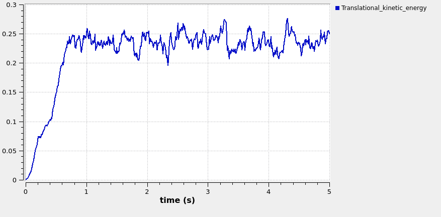
The graphs below show the particle number and the kinetic energy as a function of time, as well as the fraction of the Hertz and Rayleigh timestep:

Postprocessing with Paraview

After the simulation is completed, all data written with the output_settings command can be visualized automatically by going to the Visualization view and hitting the “Start Paraview” button.

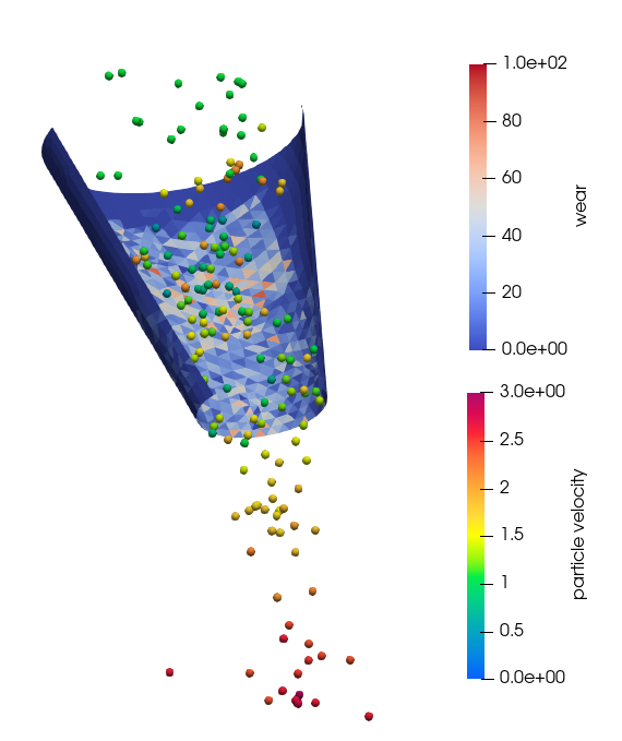
The image below shows the final state of the system, where the particles and the mesh are colored respectively with the velocity and the wear.

Case 2: Multisphere particles

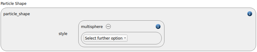
We start with cloning the initial simulation and renaming the clone to “Multisphere”. In the General Settings tab the particle_shape sphere is changed to multisphere:

One can either use an existing multisphere particle or use the Multisphere Builder (Button, or Tools/ Non-spherical Particles / Multisphere Builder) to define a new particle:

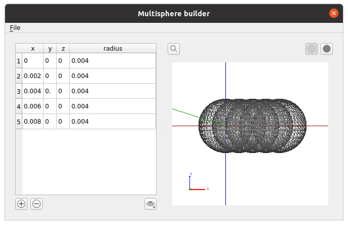
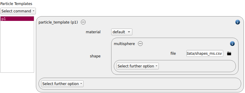
This multisphere file can be saved to a location of your choice and used for the particle template:

For nonspherical particles we add the keyword “orientation random” to the insertion command:

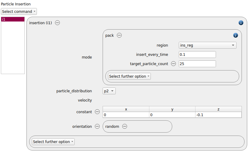
Without this keyword all nonspherical particles are inserted with the orientation that is defined by the particle template.

A test run with the existing timestep shows that the Rayleigh fraction is slightly above 0.1, which is perfectly tolerable. To avoid the constant output of warnings, we increase the tolerance of the check timestep command to 0.11 for the Rayleigh fraction:

We save the case and launch the simulation. The graphs below show the particle number and the kinetic energy as a function of time, as well as the fraction of the Hertz and Rayleigh timestep:

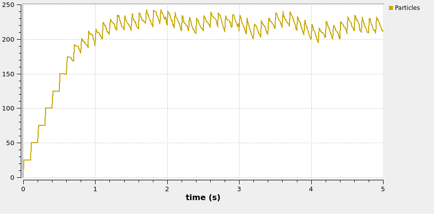
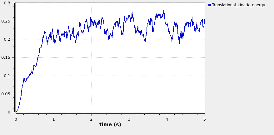
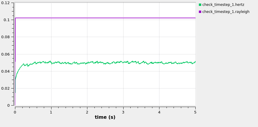
Please note, that the number of particles in this case is the number of spheres in the simulation, not the number of multisphere particles.

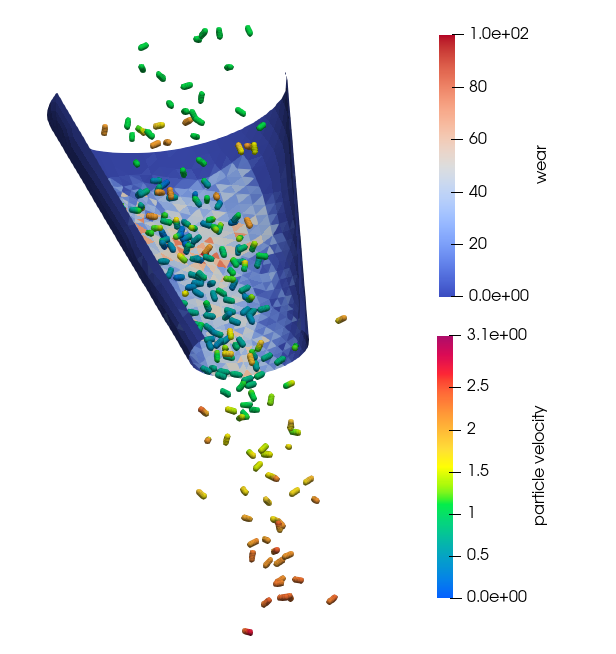
By pressing the “Start Paraview” button the data is automatically loaded in Paraview. The image below shows the final state of the system, the particles are colored according to velocity and the mesh shows the wear.

Case 3: Tablets (Superquadric particles)

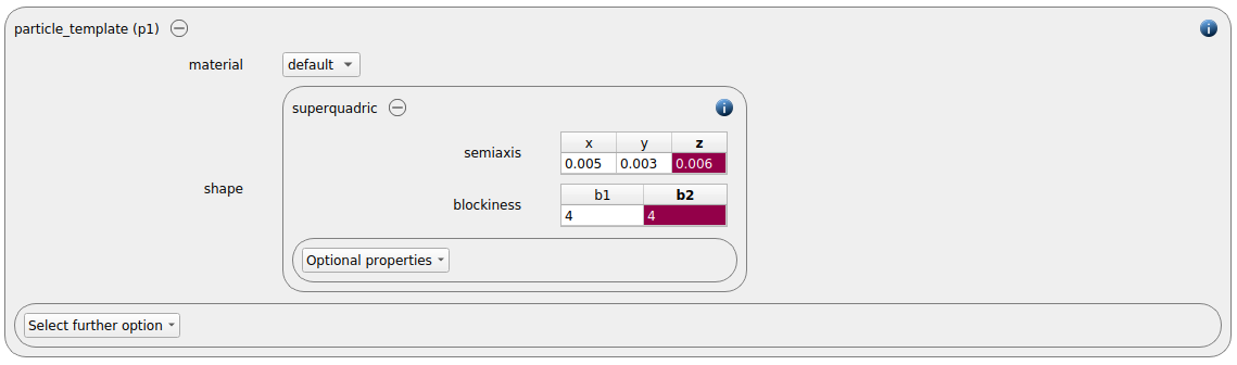
The group of superquadric particles is suitable for representing many different shapes, from tablets to (almost) cylinders and cubes etc. We make yet another clone of the spherical base case and change the particle_shape to superquadric:

Superquadric particles can either be defined directly in the particle template, or one can use the Superquadric Builder, that also visualizes the shape (Button, or Tools/ Non-spherical Particles / Superquadric Builder).

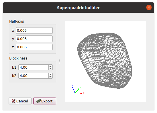
By clicking on the “Export” button, Aspherix GUI automaticall generates a new particle template. In this case, however, we replace the existing spherical particle template:

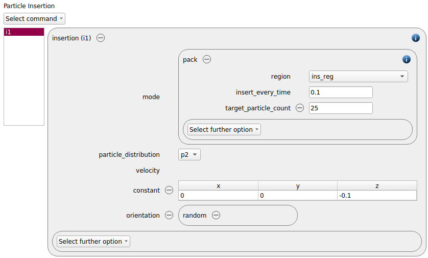
Again, we ad the keyword “orientation random” to the insertion command:

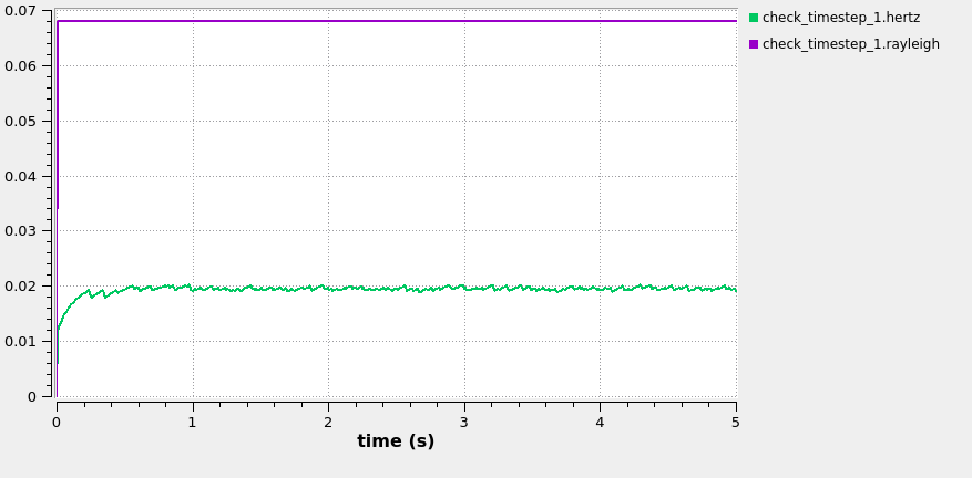
A test run of this case with the existing time step shows that the Rayleigh and Hertz timestep are clearly above 0.1. This requires us to decrease the time step from 5e-5 to 2.5e-5:

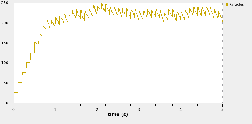
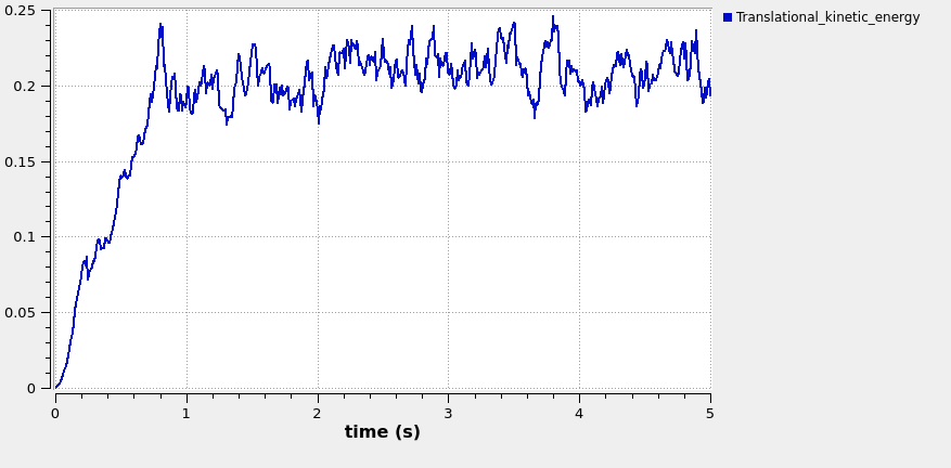
We save the case and launch the simulation. The graphs below show the particle number and the kinetic energy as a function of time, as well as the fraction of the Hertz and Rayleigh timestep:

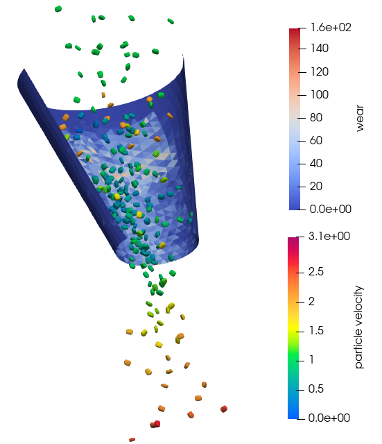
By pressing the “Start Paraview” button the data is automatically loaded in Paraview. The image below shows the final state of the system, the particles are colored according to velocity and the mesh shows the wear.

Case 4: Fibers

In this case we want to use flexible particles - so called fibers. Like a multisphere, the objects are defined by spheres, but in this case there are flexible bonds between the spheres. A fiber can only consist of a linear chain of spheres in one prinzipal direction (x, y or z), and depending on the properties and the surrounding forces fibers can also break. Fibers can be defined with overlapping and non-overlapping spheres, but the overlap cannot exceed the radius of the single sub-spheres.

We start with a clone of the spherical base case and change the particle shape:

The definition of the bonds between the sub-spheres is triggered by the usage of the cohesion model fiber:

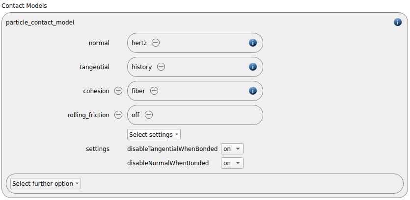
If the spheres in a fiber overlap, please add the options “disableTangentialWhenBonded on” and “disableNormalWhenBonded on”.

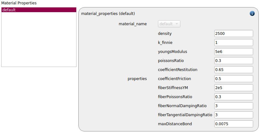
The fiber model requires additional material properties, namely a Youngs Modulus and a Poisson ratio for the fibers, a fiber normal and tangential damping ratio and a distance that defines the maximal distance that a bond can cover (i.e., when all particles overlap as planned in this case one must make sure that the parameter is larger or equal to the distance of two neighboring particles and small than the distance of a particle and its next but one neighbor).

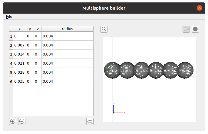
Just as for for multispheres the multisphere builder can be used to generate a fiber:

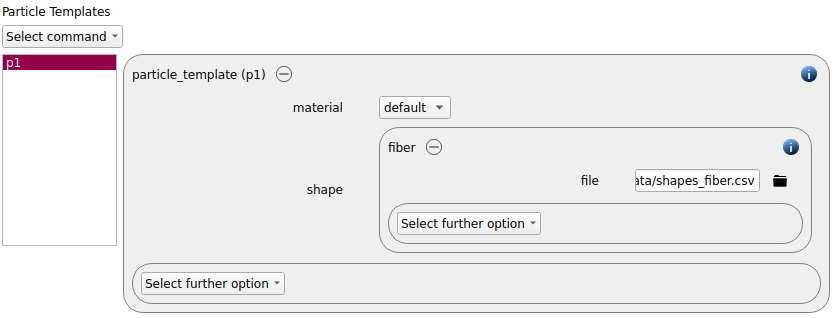
This time we use a particle template of type fiber:

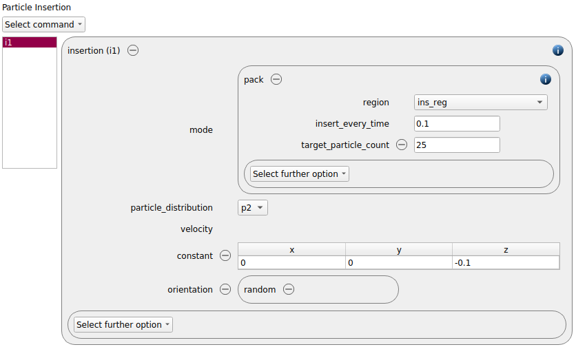
Again, the keyword “orientation random” is added to the insertion command:

Like in the multisphere case, a short run check shows that the Rayleigh fraction exceeds 0.1 slightly. By settings the check-threshold to 0.11 we can avoid related warnings:

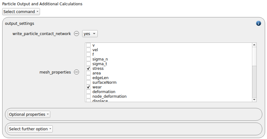
In this case we visualize the contacts between the particles by adding the property write_particle_contact_network yes to the output_settings command:

We save the case and launch the simulation. The graphs below show the particle number and the kinetic energy as a function of time, as well as the fraction of the Hertz and Rayleigh timestep:

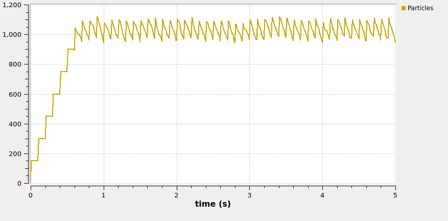
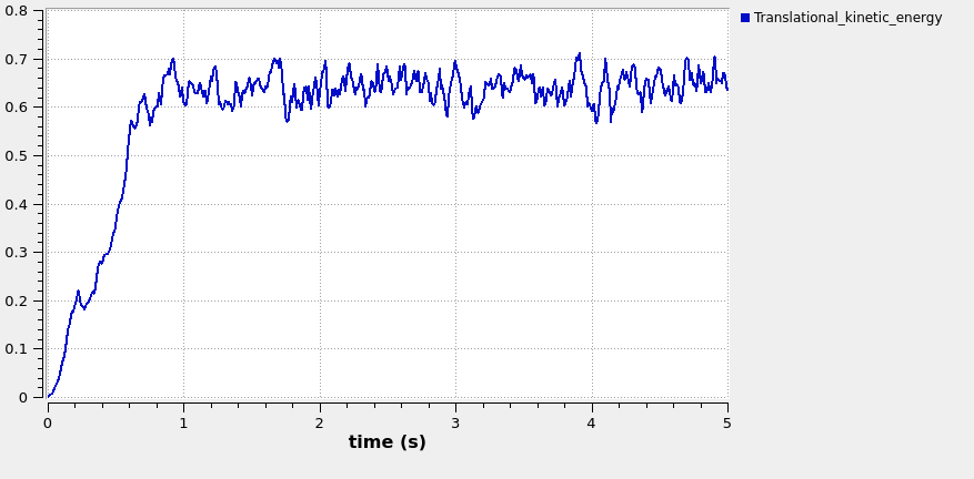
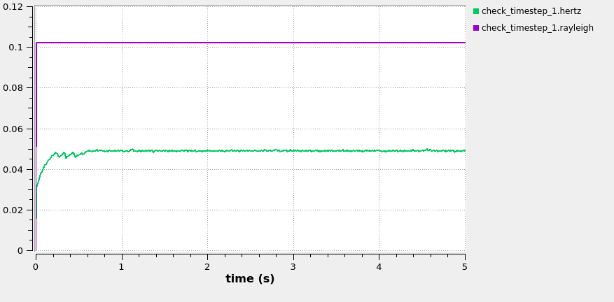
The number of particles represents the number of spheres in the simulation, not the number of fibers.

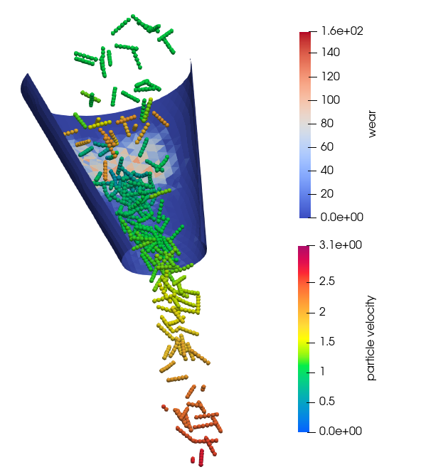
By pressing the “Start Paraview” button the data is automatically loaded in Paraview. The image below shows the final state of the system, the particles are colored according to velocity and the mesh shows the wear.

Case 5: Facetted particles (Convex)

For simulations with convex facetted particles we require the particle geometry as strictly convex stl file. In case you need help with generating such a file, please contact DCS, we have tools that can help with this task.

We start with a clone of the basic sphere case and change the particle shape to convex:

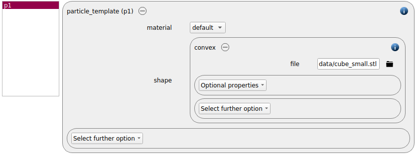
We use the mesh of a small cube (0.01 m side length) for the definition of the particle template.

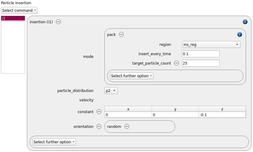
Again, the keyword “orientation random” is added to the insertion command:

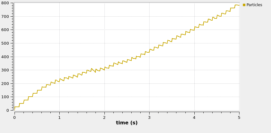
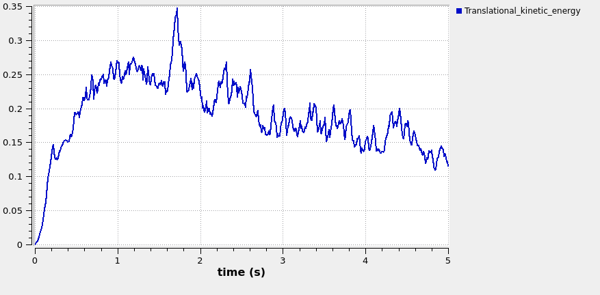
We save the case and launch the simulation. The graphs below show the particle number and the kinetic energy as a function of time, as well as the fraction of the Hertz and Rayleigh timestep:

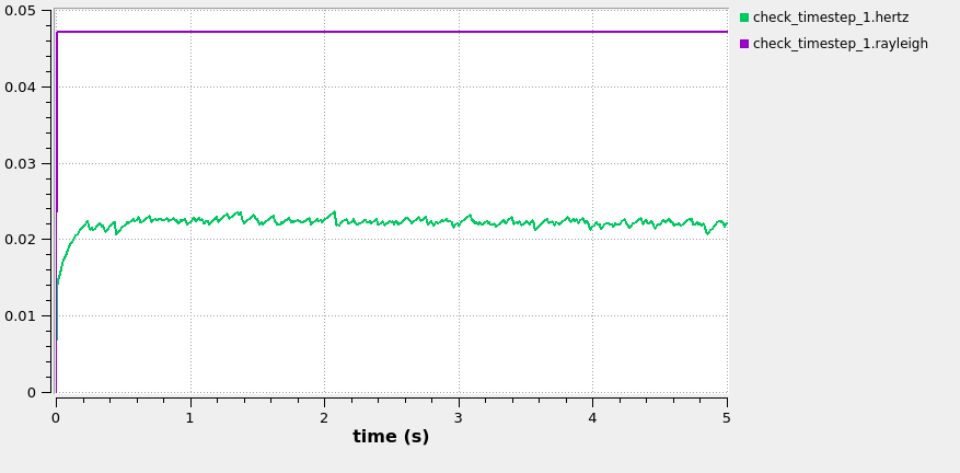
By pressing the “Start Paraview” button the data is automatically loaded in Paraview. The image below shows the final state of the system, the particles are colored according to velocity and the mesh shows the wear.

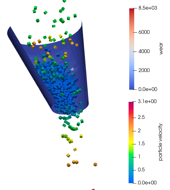
Case 6: Facetted particles (Concave, arbitray shapes)

For simulations with non-convex particles we require an stl file of the geometry as input. The shape has to be cut into convex blocks that are automatically connced to each other in Aspherix. We provide a tool that converts an arbitrary concave particle into the required decomposition and provides a shape file for the particle template.

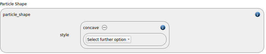
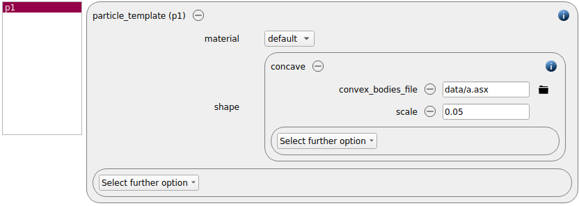
We start with a clone of the basic sphere case and change the particle shape to concave:

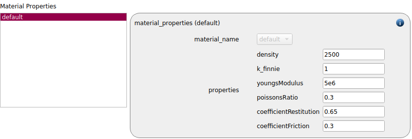
Since particles with different shapes obviously behave differently, we are reducing the coefficient of friction to 0.3 - with this we avoid a too large particle pile on the chute:

The particle that we want to use in this case is a letter “A”. We do not want to provide a manually generated decomposition (would be possible), but we want Aspherix to generate the required format. We use the Concave Builder (button or Tools / Non-spherical particles / Concave Builder) for this task:

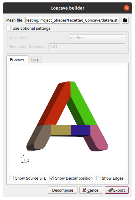
We select our stl file, keep the standard settings and click “Decompose”. Depending on the complexity of the the provided mesh this can take a while. Once completed, the new decomposition can be exported to a particle template. Please make sure that the case is already saved with its new name - this ensures that the relative path in the particle template is correct:

Again, the keyword “orientation random” is added to the insertion command:

We save the case and launch the simulation. The graphs below show the particle number and the kinetic energy as a function of time, as well as the fraction of the Hertz and Rayleigh timestep:

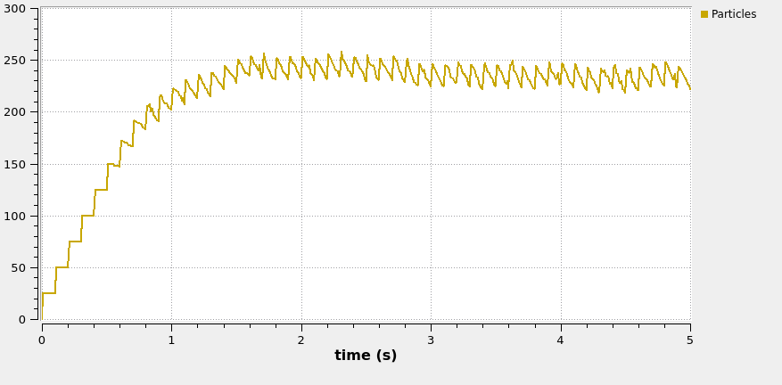
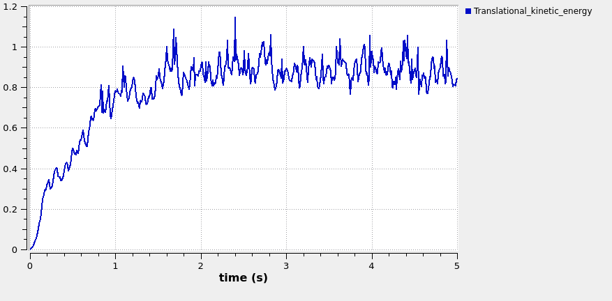
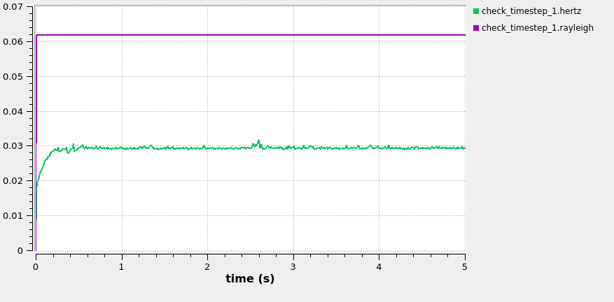
The number of particles represents the number of convex parts in the simulation, not the concave objects.

By pressing the “Start Paraview” button the data is automatically loaded in Paraview. The image below shows the final state of the system, the particles are colored according to velocity and the mesh shows the wear.

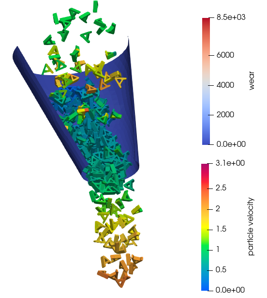
In this tutorial we demonstrated the simplicity of changing sphere types in simulations. Please note that different shapes might required different time steps, and in some cases also special settings (fiber parameters, switching off normal / tangential force for spheres that are bonded, radom orientation of particles during the insertion, …). The image below shows the final results for all cases next to each other. Please note that the materials deviate strongly (in shape and mass, partially also in parameters), which obviously leads to different wear values.