 Home
HomeDEM simulation with superquadric particles
This tutorial shows how to run simulations with superquadric particles.
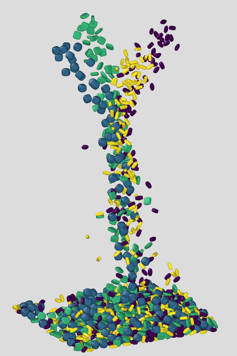
Name of the case: Project_Superquadrics
Setting up the Aspherix(R) GUI simulation
As a first step, the used materials command as well as the simulation domain are defined in the General Settings tab. Please note that in case of multiple dependent simulations, the dimensions of the simulation domain can only be defined in the first simulation. This means that the box forming the simulation domain has to be chosen big enough from the beginning.
General settings
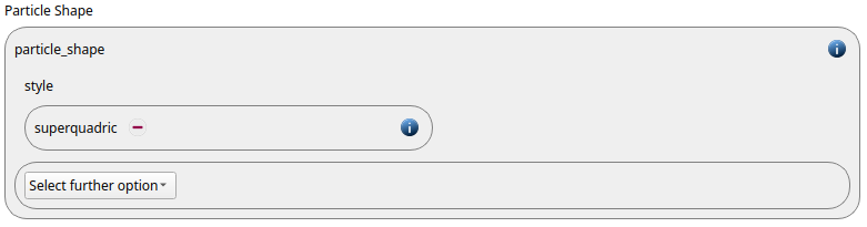
In this simulation we set particles of particle_shape command superquadric:
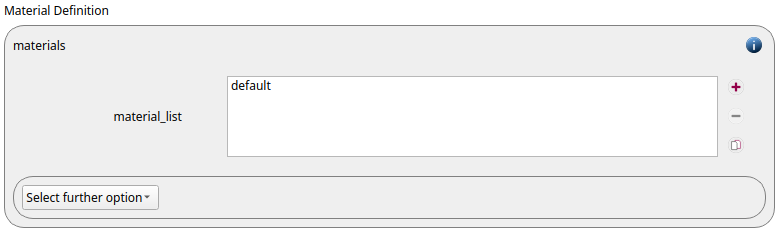
In this simulation only one material type is used (here called default):
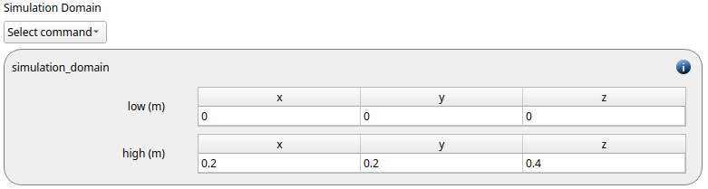
The simulation_domain command with x and y dimensions ranging from 0 to 0.2 and z dimension ranging from 0 to 0.4 is created:
Meshes and regions
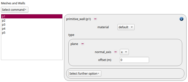
The side and bottom walls are set by five primitive walls of
type plane with the following properties:
Name |
Normal axis |
Offset |
p1 |
x |
0 |
p2 |
x |
0.2 |
p3 |
y |
0 |
p4 |
y |
0.2 |
p5 |
z |
0 |
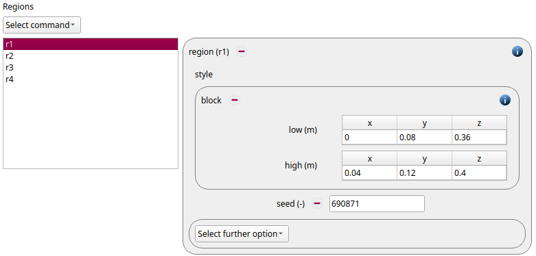
Later on, four templates of superquadric particles will be inserted. For this purpose, we define four different block regions:
Name |
Low (x, y, z) |
High (x, y, z) |
r1 |
(0, 0.08, 0.36) |
(0.04, 0.12, 0.4) |
r2 |
(0.16, 0.08, 0.36) |
(0.2, 0.12, 0.4) |
r3 |
(0.08, 0, 0.36) |
(0.12, 0.04, 0.4) |
r4 |
(0.08, 0.16, 0.36) |
(0.12, 0.2, 0.4) |
Physics models
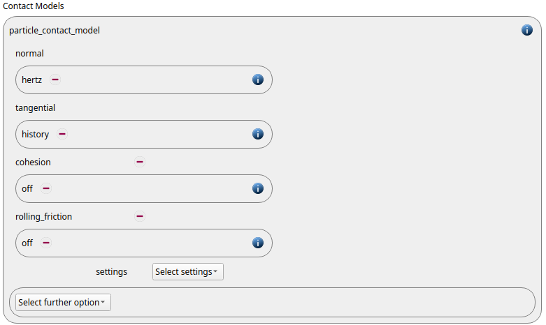
The contact models are now defined. For the particles we use the normal contact model hertz and the tangential model history:
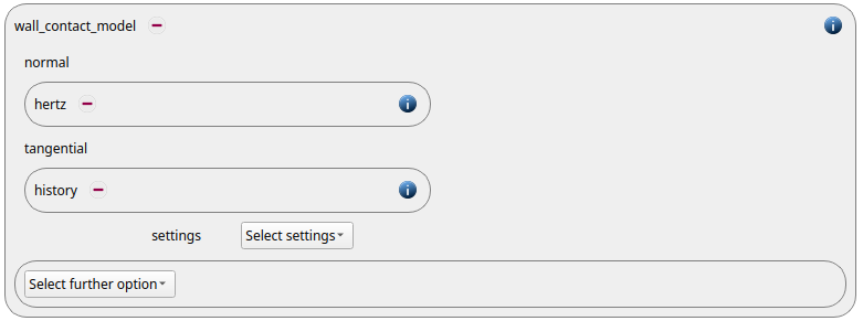
Since we added primitive walls in the previous section, a wall contact model is also added automatically to this section. We use the normal contact hertz and the tangential model history:
Finally, the gravity is enabled:

Per default the gravity has a magnitude of 9.807 and acts into negative z-direction. These defaults can be changed by either setting the magnitude or the direction manually.
Particles
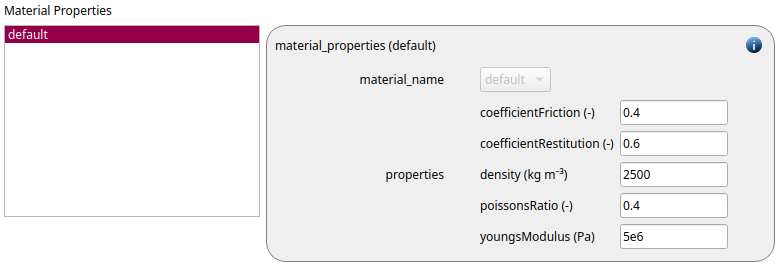
In the general settings tab we only defined a single material type (default), whose settings have to be specified here:
default |
|
density |
2500 |
Young’s modulus |
5e6 |
Poisson’s ratio |
0.4 |
Coefficient of restitution |
0.6 |
Coefficient of friction |
0.4 |
We will use the superquadric builder to generate the particle shapes, so we remove the default particle distribution and template. The superquadric builder can be accessed through Tools / Non-spherical particles / Superquadtric builder or the respective button in the symbol bar.
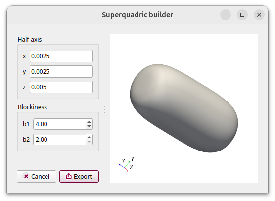
The “Export” button adds the template to the active simulation.
We create four particle templates with the following properties:
name |
shape 1 |
shape 2 |
shape 3 |
blockiness 1 |
blockiness 2 |
p6 |
0.025 |
0.0025 |
0.0005 |
4 |
2 |
p7 |
0.005 |
0.005 |
0.005 |
3 |
3 |
p8 |
0.005 |
0.002 |
0.005 |
4 |
4 |
p9 |
0.005 |
0.002 |
0.002 |
4 |
4 |
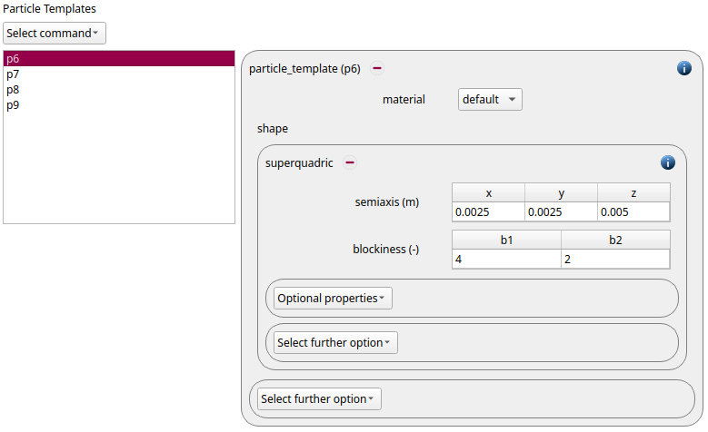
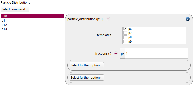
The four templates are used to create four different particle distributions, which consist of one template each:
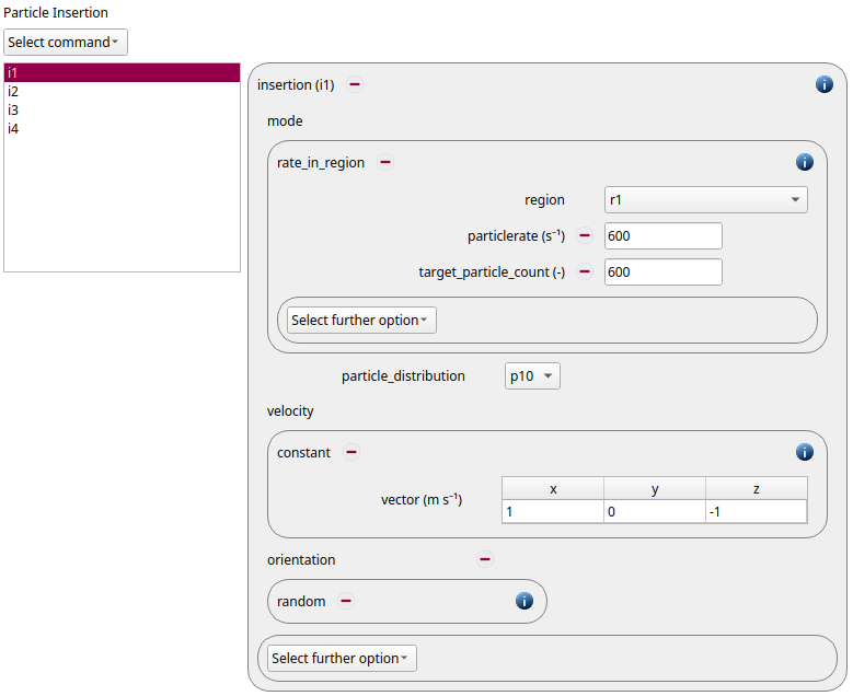
The final step is the definition of the insert commands. Four insertion command commands of mode rate in region are used with random orientation. The number of particles, particle rate, insertion region and insertion velocity are given the following:
name |
nparticles |
particlerate |
vx |
vy |
vz |
region |
i1 |
600 |
600 |
1 |
0 |
-1 |
r1 |
i2 |
300 |
300 |
-1 |
0 |
-1 |
r2 |
i3 |
500 |
500 |
0 |
1 |
-1 |
r3 |
i4 |
600 |
600 |
0 |
-1 |
-1 |
r4 |
Simulation control
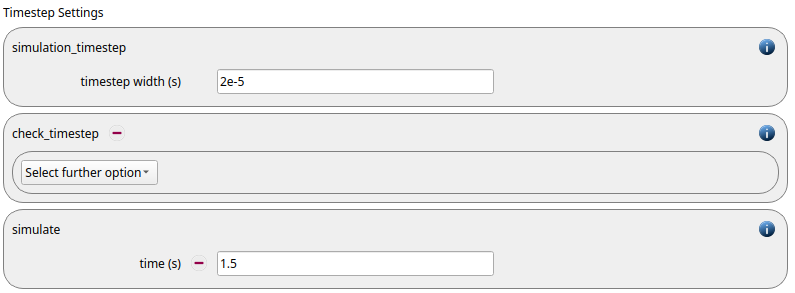
In this tab, we first define the time-step settings such as the simulation timestep of 1e-5 seconds and the total simulation time of 1.5 seconds.
Per default also the check_timestep command command is enabled, which calculates the Hertz and Rayleigh time and outputs a warning if the time step exceeds 10 %.
Output settings
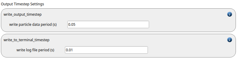
In this tab, we first define the time-step width for the file and the terminal output:
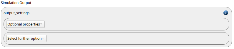
The output_settings command command controls the writing of all particle data as well as the geometries. In addition, it triggers the output of global quantities such as the kinetic energy of the particles or total normal and shear stresses onto meshes.
Running the simulation
After completing the setup and saving it, the simulation can be launched. To do so, switch to the Simulation view and start the run by clicking Start. The simulation is executed in parallel using MPI on four cores:
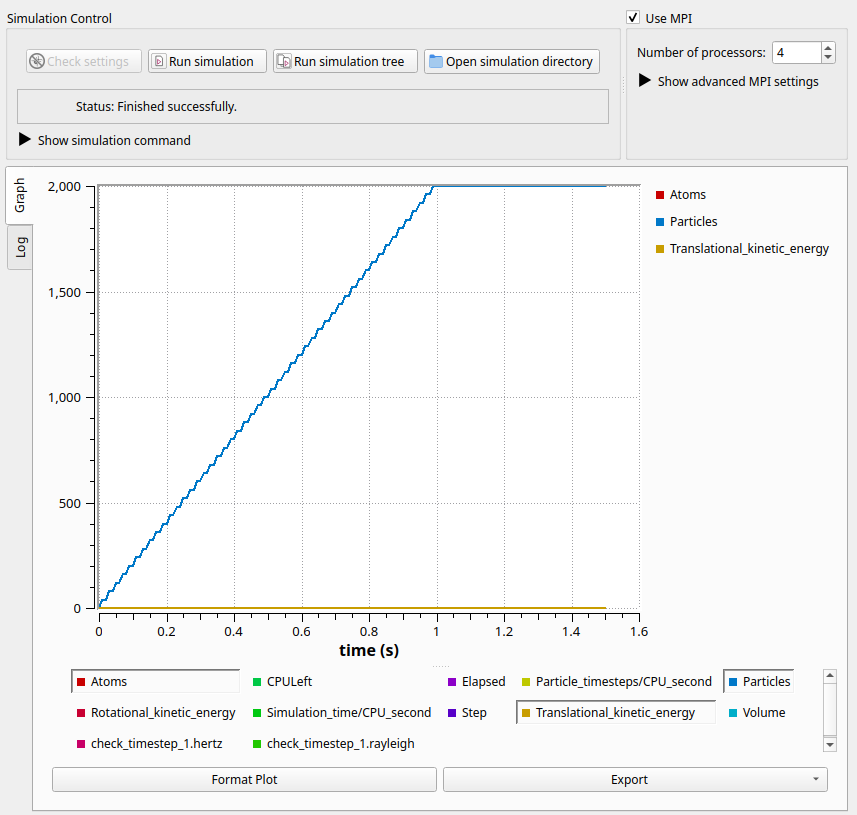
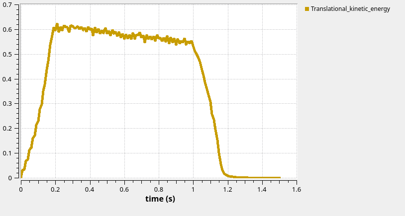
This graph shows the kinetic energy in the system during the simulation:
Postprocessing
Change to the visualization tab to open the results with Paraview or Ovito: