Home
HomeRotating drum with A and X-shaped concave particles
In this tutorial we insert A and X-shaped particles into a drum, which is subsequently rotated.
Name of the case: Project_AX_Rotating_Drum
This case involves two simulations: the initial simulation for insertion of the particles, and a second derived simulation for rotating the drum.
Particle insertion
As a first step, the particle shape, the used material and the simulation domain are defined in the General Settings tab. Please note that in the case of multiple dependent simulations, the dimensions of the simulation domain can only be defined in the first simulation. This means that the box forming the simulation domain has to be chosen big enough from the beginning in case you have moving meshes that might leave the domain.
General settings
In this simulation we set particles of particle shape concave:

We define two materials command, using the default names:

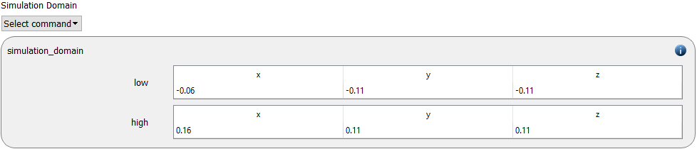
The simulation domain is defined next, with x between -0.06 and -0.16, and y and z ranging from -0.11 to 0.11:
Meshes and regions
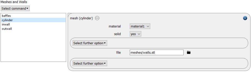
The geometry is composed of meshes, which we insert via the mesh command command. We need to insert the cylinder which makes the drum casing:
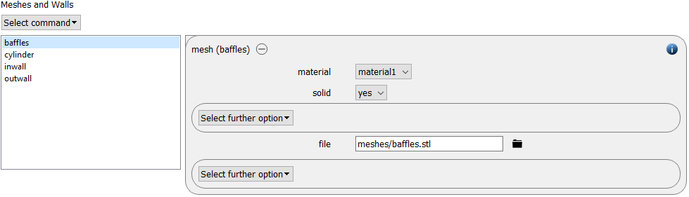
The baffles inside the drum for mixing:
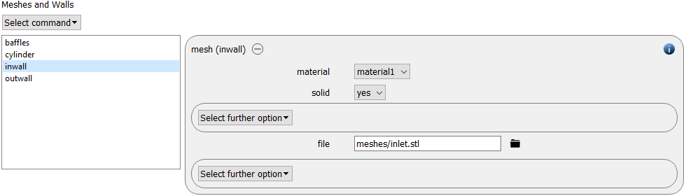
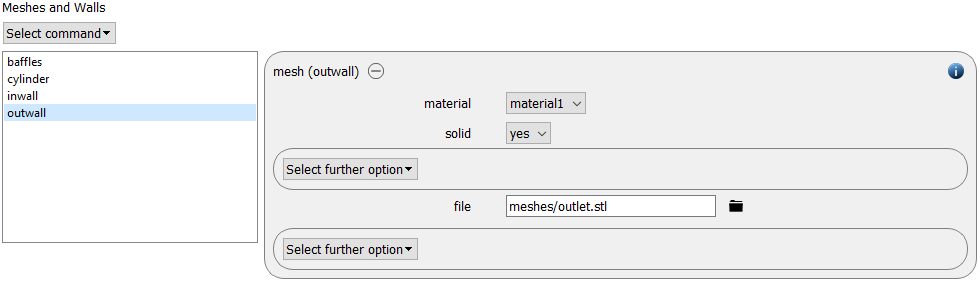
And the two closures at either side of the drum, which we call inwall and outwall:
Physics models
The contact models are now defined. For the particles we use the normal contact model hertz and the tangential model history:
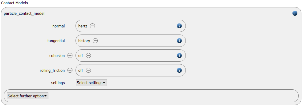
Since we added meshes in the previous section, a wall contact model is also added automatically to this section. We use the same properties as for the particle contact model:
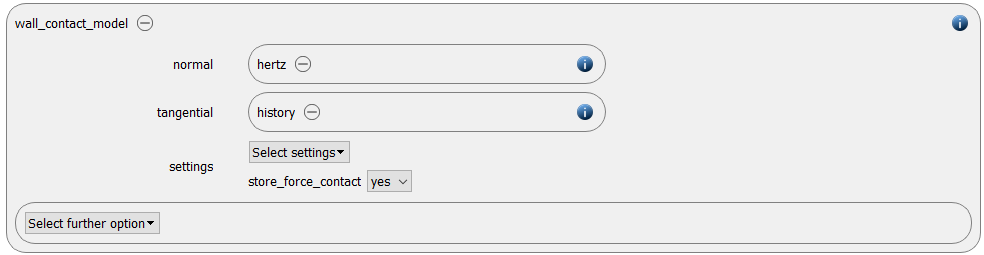
Please note that for convex and concave simulations the setting store_force_contact has to be set to yes.
Finally, gravity is enabled:

By default the gravity has a magnitude of 9.807 and acts into negative z-direction. These defaults can be changed by either setting the magnitude or the direction manually.
Particles
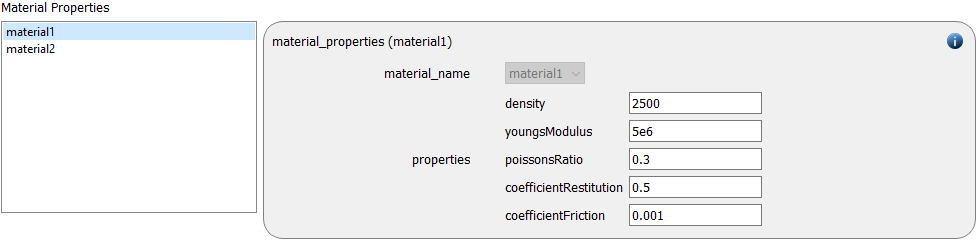
In the General Settings tab we defined two material types, which use the same properties as shown in the table below:
Property |
value |
Density |
2500 |
Young’s modulus |
5e6 |
Poisson’s ratio |
0.3 |
Coefficient of restitution |
0.5 |
Coefficient of friction |
0.001 |
These properties are defined in this step, in the Particles tab. Since both materials use the same properties, one is shown as an example:
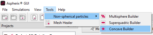
A particle template for concave particles consists of a set of convex bodies. Aspherix automates the process for generating convex bodies from concave shapes with the Concave Builder, which can be accessed via the Tools menu:
The Concave Builder loads an STL file for the concave particle and decomposes it automatically into convex shapes. The STL can be loaded in the “Mesh file” input in the tool and visualized in the Builder(the files are available in the data folder of the tutorial).
The file is decomposed by selecting “Decompose” at the bottom of the window. After decomposition, the decomposed file can be visualized in the Builder (you may need to de-select “Show Source STL” to visualize it properly). The figures below show the original STL and decomposed versions of both concave particles used in this tutorial:
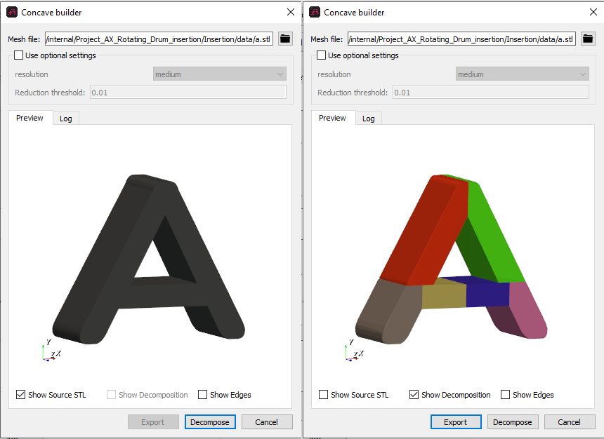
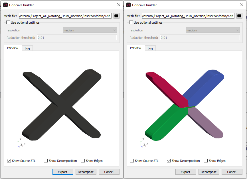
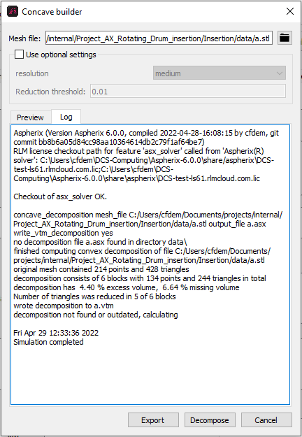
After decomposition, clicking “Export” will export the files for the decomposed convex shapes to the folder where the STL is located. The convex bodies will be used in the particle templates below. The Builder also offers a log of the decomposition in a separate tab:
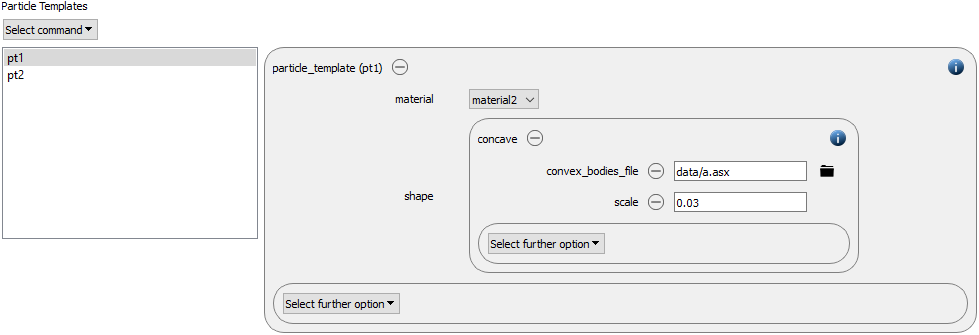
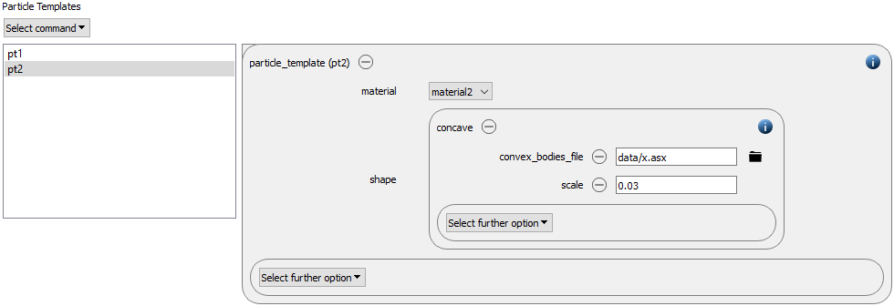
We now add the particle templates of style concave and with a scale of 0.03. Note the files loaded with the extension ASX, which were generated by the Concave Builder:
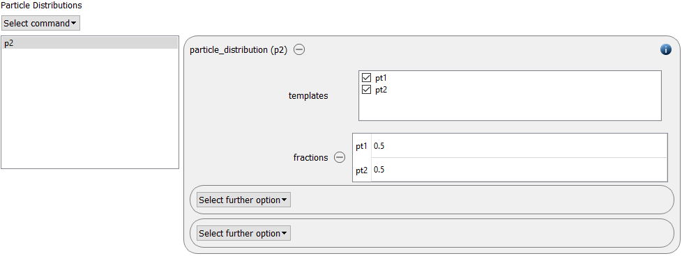
The templates are used for a particle distribution composed of 50% of each template:
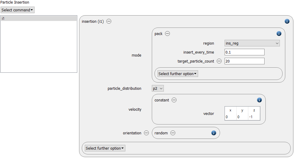
A pack of particles with a velocity of 1 m/s in negative z-direction and target_particle_count of 20 is inserted every 0.1 s using an insertion command command with mode pack. The orientation is set to random:
Simulation control
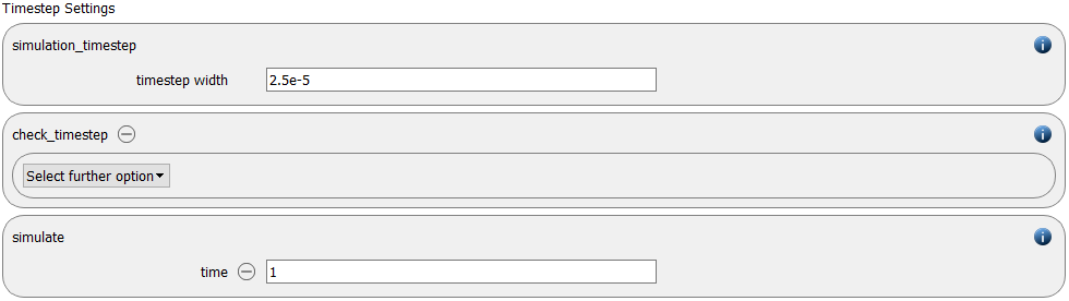
In this tab, we first define the time-step settings such as the desired simulation timestep of 2.5e-5 seconds and the total simulation time of 1 second. By default also the check_timestep command command is enabled, which throws a warning when the time step exceeds 10 % of the Rayleigh or the Hertz time. These thresholds can be changed by setting an alternative value for hertz_fraction or rayleigh_fraction.
Here we can also enable loadbalancing to allow Aspherix to optimize CPU usage:

Output settings
In this tab we first define the timestep width for the file and the terminal outputs:

The output_settings command command takes care that all particle information and the meshes are written to files accordingly. Furthermore it triggers the output of global quantities such as the kinetic energy of the particles or total normal and shear stresses onto meshes to the terminal. Please note that if the output of per-cell information on meshes such as wear, velocity of stress are desired, one has to add the keyword mesh_properties and select the required output.

Running the simulation
After completing the setup and saving it, the simulation can be launched. Hence, change to the Simulation view. First hit the “Check settings” button, and if the check returns “Check settings successfully completed” the simulation can be run by hitting “Start”.
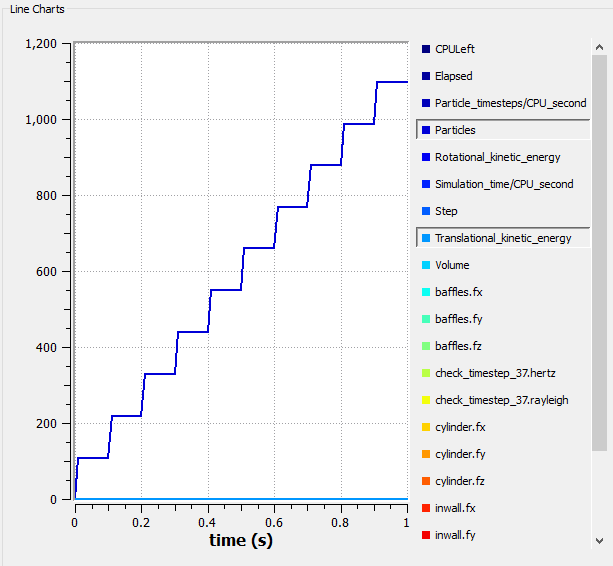
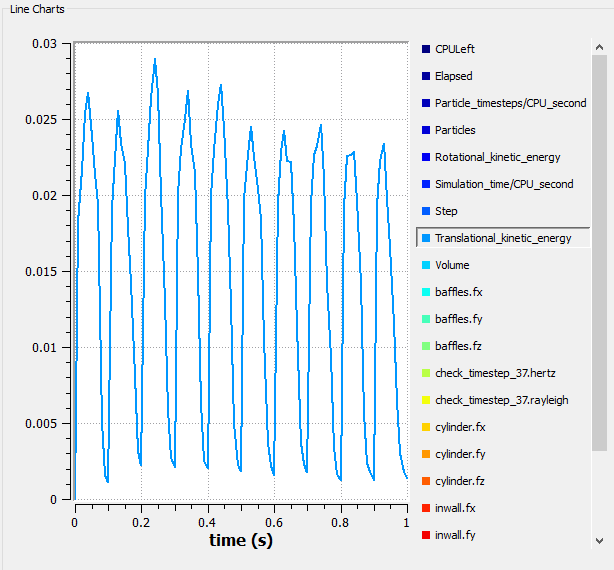
Particle number increases every 0.1 s as new particles are inserted. Similarly, kinetic energy oscillates, increasing when particles are added and reducing as they begin to settle.
Postprocessing with Paraview
After the simulation is completed, all data written with the output_settings command command can be visualized automatically by going to the Visualization view and hitting the “Start Paraview” button.
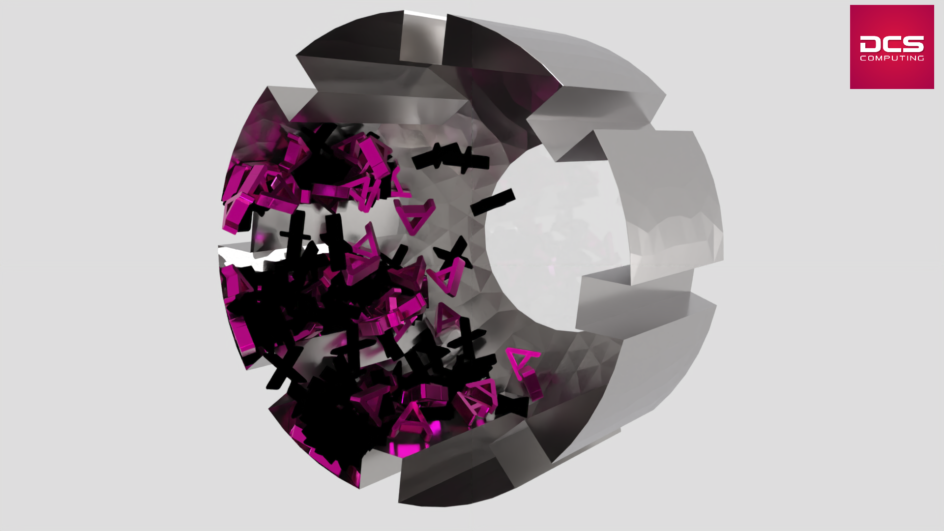
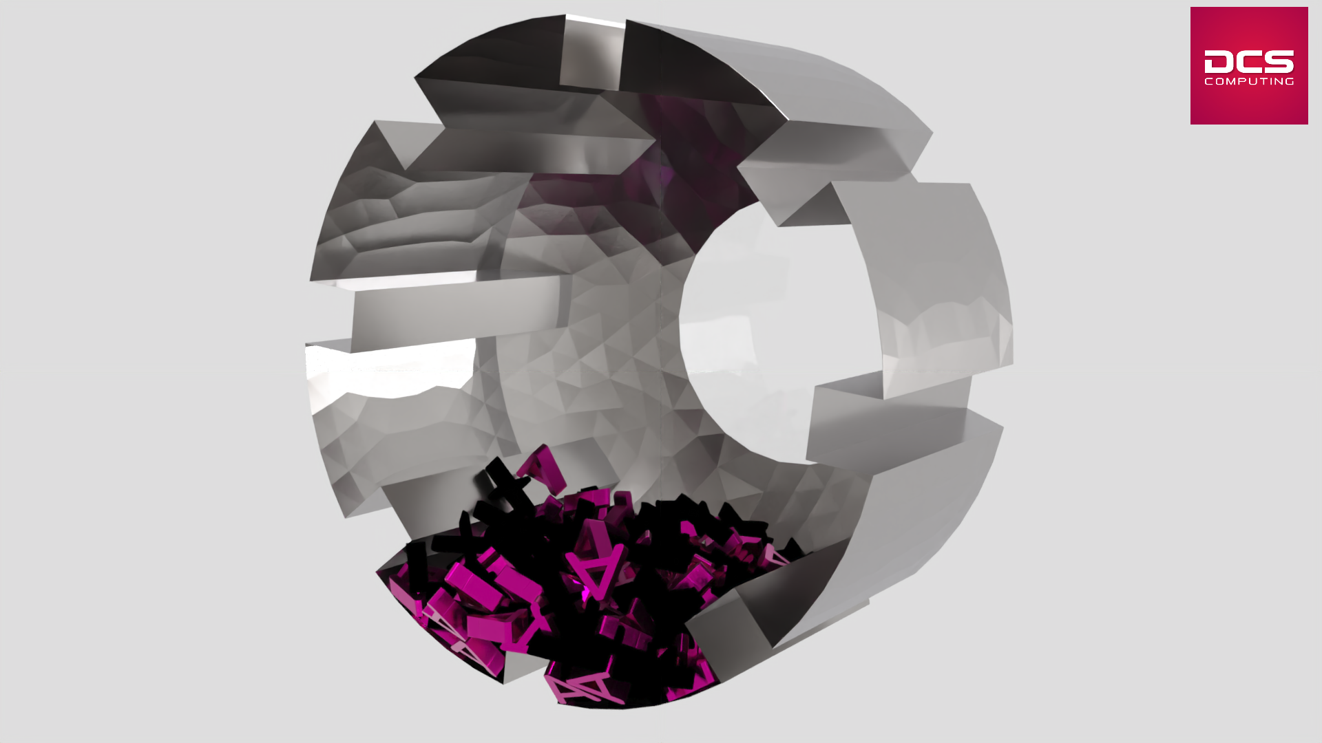
The image below shows the simulation state after 1 second of inserting particles. This is a rendered image made with Paraview.
Rotating the drum
With the particles inserted, the drum must now be rotated. For that we need to derive a simulation from the previous one, so that our project looks like this:
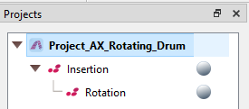
When a simulation is derived, some of the settings are locked as they depend on the previous simulation (such as simulation domain).
Setting up mesh rotation
First step is to add a mesh_module for the rotation, in the Meshes and Regions tab. We set the origin and axis of rotation and a period of 2 seconds:
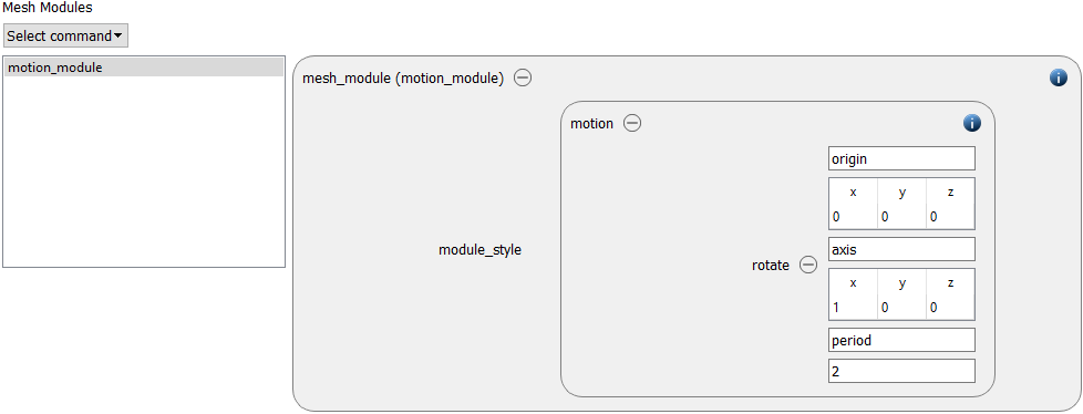
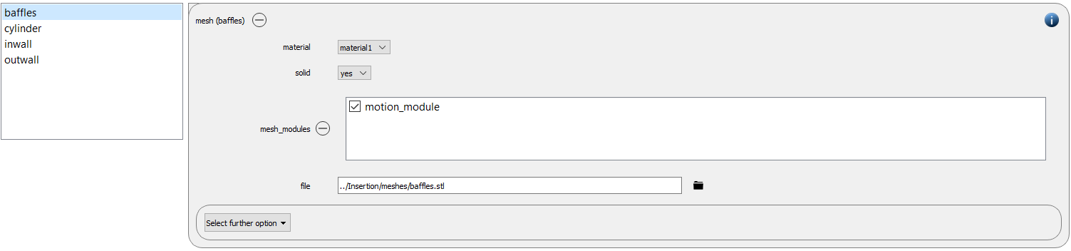
This mesh_module must be applied to all the meshes, as in the example in the figure:
Removing the particle insertion command
Since no further particles will be inserted, the insertion commands as well as particle distribution, and insertion region can be deleted. Please note that a command can only be deleted if no other command depends on it. Therefore the mentioned order has to be kept when removing all insertion-related components. The particles tab will then contain only the particle properties and templates.
Simulation control
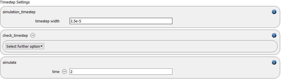
For this simulation, we keep the timestep of 2.5e-5 and increase the simulation time to 2 s:
Running the simulation
After adjusting the setup and saving it, the simulation can be launched. Change to the Simulation view. As before, first hit the “Check settings” button, and if the check returns “Check settings successfully completed” the simulation can be run by hitting “Start”.
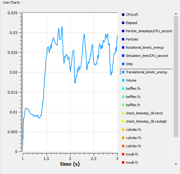
For this simulation, since no more particles are inserted, the number of particles in the simulation remains constant. The kinetic energy, however, will quickly increase as the drum starts rotating, and then changes as particles tumble inside the drum.
Postprocessing with Paraview
As before, you can go to the Visualization view and hit the “Start Paraview” button to visualize the results in Paraview.
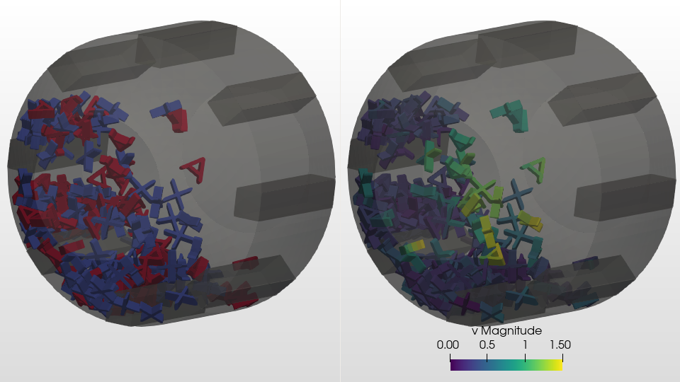
The image below shows the simulation state after 2 seconds after the drum starts its rotation, the coloring on the left is chosen according to the mass to highlight the two particle types, while on the right velocity is used.