Simulation Setup

CPU vs. GPU

Aspherix® GUI allows you to set up simulation cases for either CPU or GPU execution. Because the available feature sets differ between these two modes, the first step when creating a new case is to choose whether it will run on the CPU or the GPU. Please note that this selection cannot be changed later.

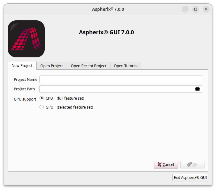
For CPU-based calculations, the complete Aspherix® feature set is available. To get started, refer to the various tutorials.

For GPU-based cases, a streamlined, GPU-optimized feature set is provided. Please consult the corresponding tutorials for examples and guidance.

Mesh Generation Tab

In Standard Mode this tab is only visible if the simulation is not appified. This tab contains the “Start Salome” button, which launches the CAD and meshing tool if the path is defined correctly (see options_). Alternatively, also other pre-processing tools can be linked to this button if preferred. Aspherix® requires stl meshes for surfaces and vtk meshes for volumes. Several options for improving the mesh quality and increasing the tolerance for mesh handling are available within Aspherix® (see e.g., Mesh healer).

Additional Tools

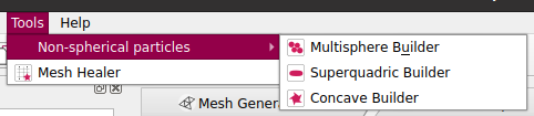
The tools section of Aspherix® GUI contains a set of little helpers for generating non-spherical particles (superquadric particles, multispheres and concave particles) and for improving the mesh quality:

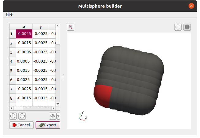
Multisphere Builder

The “Multisphere Builder” can be used to generate, save, load and visualize multisphere particles. The particles can be saved as *.txt or *.csv file and then be used as “file” in the multisphere particle templates of the simulation.

Superquadric Builder

The “Superquadric Builder” can be used to generate and visualize superquadric particles and for exporting them to the current simulations.

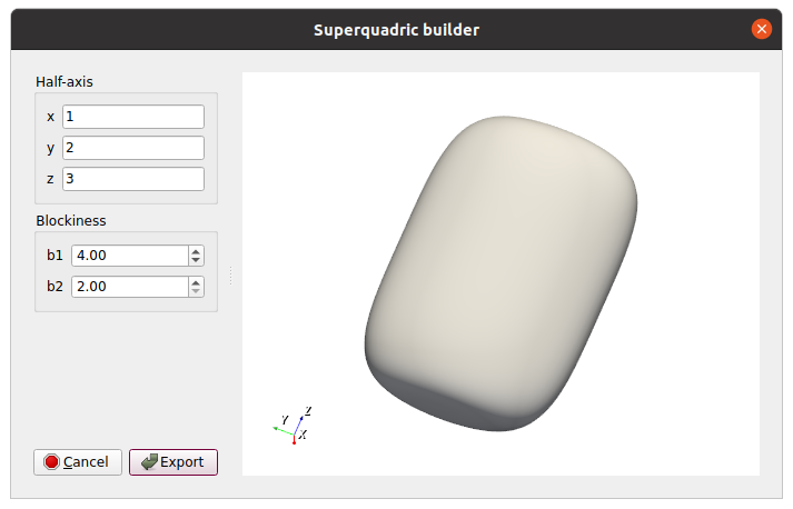
Superquadric particle templates are currently not saved in files, but defined directly in the according particle template command. The “SQ Builder” can only be used inside simulations.

Concave Builder

Aspherix® automates the process for generating convex bodies from concave shapes using the Concave Builder, which converts user-defined STL files into a decomposition compatible with Aspherix® Solver. The Concave Builder can only be used within simulations that have already been saved as it requires an existing folder structure.

The Concave Builder allows you to load an STL file of the concave particle through the Mesh file input and visualize it within the Builder (example files are available in the tutorial’s data folder). The STL is then automatically decomposed into convex shapes by selecting Decompose at the bottom of the window. After decomposition, the resulting convex shapes can be visualized in the Builder - note that you may need to deselect Show Source STL for proper visualization.

The figure below shows the original STL alongside the decomposed versions of an example concave particle:

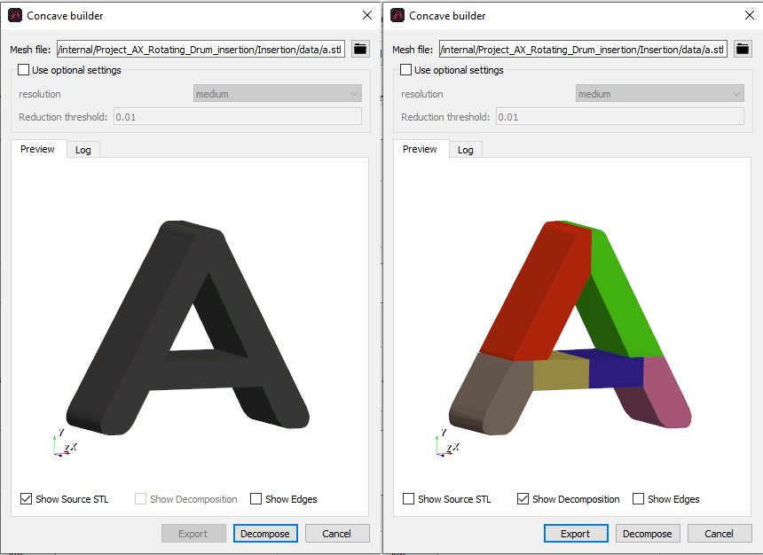
After decomposition, clicking “Export” saves the files for the decomposed convex shapes as well as the stl file to the data folder of the simulation and creates a new particle_template that uses the shape.

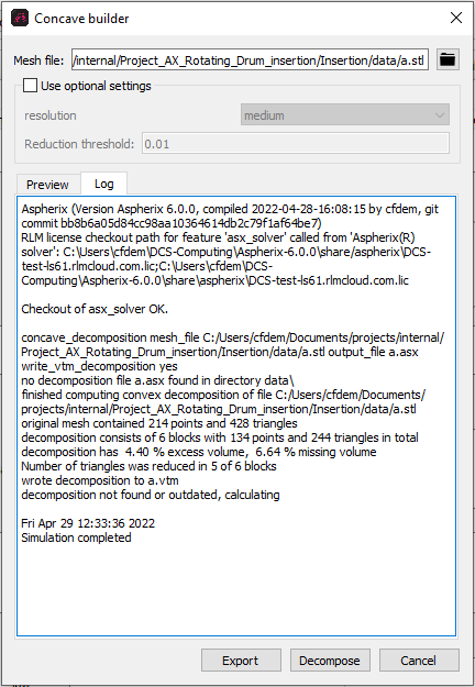
The Builder also provides a log of the decomposition process in a separate tab:

Mesh Healer

DEM simulations do not strictly require watertight meshes, as long as any holes are sufficiently small. The mesh command (DEM Setup / Meshes and Regions / Surface meshes) has the option element_exclusion_list, which, in the read mode allows the user to define a list of (bad) elements to be ignored during the simulation. This list can be generated with the element_exclusion_list option in write mode, or more conveniently, with the Mesh Healer tool:

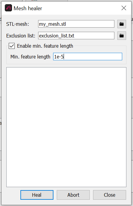
The Mesh Healer tool also allows you to define a minimal feature length. For further details, please refer to the documentation of the mesh command command.

DEM Setup Tab

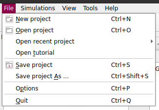
This is the core tab for setting up DEM simulations. In Standard Mode this tab is only visible if the simulation is not appified. Example case setups can be found among the tutorials. The prepared simulations can be loaded by using the “Open tutorial” functionality in the File menu:

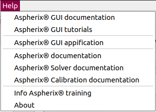
Information about the commands and their usage can be found in the Aspherix® Solver documentation, which can either be accessed by the info button next to each command or generally via Help / Aspherix® Solver documentation:

DEM App Settings Tab

This is the core tab for changing settings of appified simulations. This tab is only visible when simulations are appified and when Standard Mode is active. Concerning tutorials and the use of the help menu please have a look at the section above.

CFD-DEM Setup Tab (Linux only)

In Standard Mode this tab is only visible if the simulation is not appified. The CFD-DEM can be used as part of the setup process for a fully coupled CFD-DEM simulation:

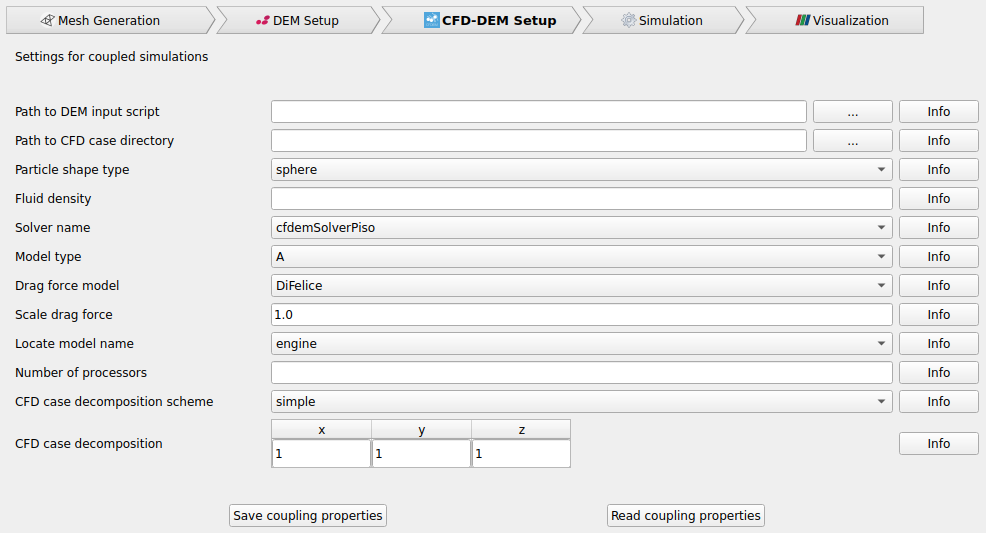
An example for such a setup process is shown in the screencast “Coupled CFD-DEM Case with Aspherix GUI”:

https://vimeo.com/manage/videos/649446884/80c7ddc864

Custom Commands

Any commands available in Aspherix® Solver but not included in Aspherix® GUI can be added to a simulation setup as custom commands in the Custom Settings tab within the DEM Setup section. The GUI organizes commands according to internal weights, which must also be specified for custom commands. The following list of weights for existing Aspherix® GUI commands can help users determine the appropriate weight for their custom command:

Command	weight	Command	weight
coarsegraining	1	calculate/wall_normal_elastic_energy	17
particle_shape	1	check_timestep	17
units	2	cundall_damping	17
boundary_conditions	3	enable_gravity	17
processors	3	enable_heat_conduction	17
read	3	enable_loadbalancing	17
simulation_domain	4	enable_sieving_for_wall_material	17
simulation_timestep	4	heat/gran/melting	17
write_output_timestep	4	heat/gran/roasting	17
write_to_terminal_timestep	4	limit_velocity	17
materials	5	calculate/dissipated_energy	18
region	5	calculate/wall_dissipated_energy	18
global_scalar	6	enable_buoyancy	18
material_interaction_properties	6	enable_cfd_coupling	18
material_properties	6	enable_surface_heating	18
neighbor_list	6	update_particle	18
custom_cohesion_model	7	addforce	19
custom_normal_model	7	addforce/magnetic	19
custom_rolling_model	7	addforce/weighted	19
custom_surface_model	7	change/size	19
custom_tangential_model	7	change/size/multisphere	19
custom_wear_model	7	change/size/superquadric	19
property/atom	7	change/size/superquadric/anisotropic	19
property/global	7	contact/atom/counter	19
group	8	contact/atom/counter/wall	19
mesh_module	8	enable_dem_drag	19
particle_contact_model	8	enable_fem_coupling	8
wall_contact_model	8	enable_one_way_coupling	19
mesh	9	enable_two_way_drag	19
primitive_wall	9	mixing	19
concave_decomposition	10	move	19
convex_body	10	(fix) multicontact/halfspace	19
define_lattice	11	(fix) powder/update	19
particle_template	11	pressure/simplistic	19
create_particles	12	set_velocity	19
particle_distribution	12	setforce	19
breakparticle/force	13	temperature/fluid/field	19
insertion	13	calculate	20
grow_particles	14	(compute) coordination_number	20
mark_inserted_particles	14	(compute) crosssection	20
mark_particles	14	(compute) mesh/area	20
detect_surface	16	(compute) reduce	20
enable_electrical_conductivity	16	(compute) reduce/region	20
integrator	16	(compute) surface	20
liquidtransport	16	(compute) velocity/mesh	20
liquidtransport/evaporation	16	viscous	20
liquidtransport/porous	16	(dump) decomposition/vtk	22
liquidtransport/sponge	16	output_settings	23
(fix) ave/euler/custom	17	delete_particles	24
(fix) ave/euler/custom/temporal	17	restart	24
calculate/cohesion_elastic_energy	17	simulate	25
calculate/normal_elastic_energy	17	write_data	26
calculate/wall_cohesion_elastic_energy	17	write_restart	100

As a guideline: general keywords for the simulation setup typically have weights between 1 and 8, while geometry- and particle-related commands fall between 8 and 13. Commands that introduce additional physics or fixes should have weights between 14 and 19. Calculate and compute commands are assigned a weight of 20, and the output_settings command has a weight of 23. The simulate command has a weight of 25. If any commands added after this require additional simulation runtime, include another simulate command with a higher weight as a custom command. Commands sharing the same weight are sorted alphabetically.

If you want to include a block of custom commands, it is recommended to place them in a separate file and incorporate it using a custom include command. Assign a weight to this command that positions the block at the desired location within the simulation setup.

Unlocking simulations

When a simulation has derived simulations, it gets locked automatically. This means that the simulation can still be run and postprocessed, but no changes can be applied. This is indicated by this symbol in the upper right corner of the DEM Setup tab:

Locked simulations can be unlocked by clicking on the lock button. The button then changes to an open lock:

Please note that as soon as unlocked simulations are changed and saved their status automatically changes to incomplete. Derived simulations can only be launched after regenerating the results of the changed simulation.

Even when unlocking simulations, only certain properties can be changed. Quantities that cannot be modified in derived simulations (e.g., size of the simulation domain, number of materials, contact models, …) are not modifiable in unlocked simulations either.