Mowing grass formed by fibers

This tutorial shows the mowing of grass, which is represented by fibers.

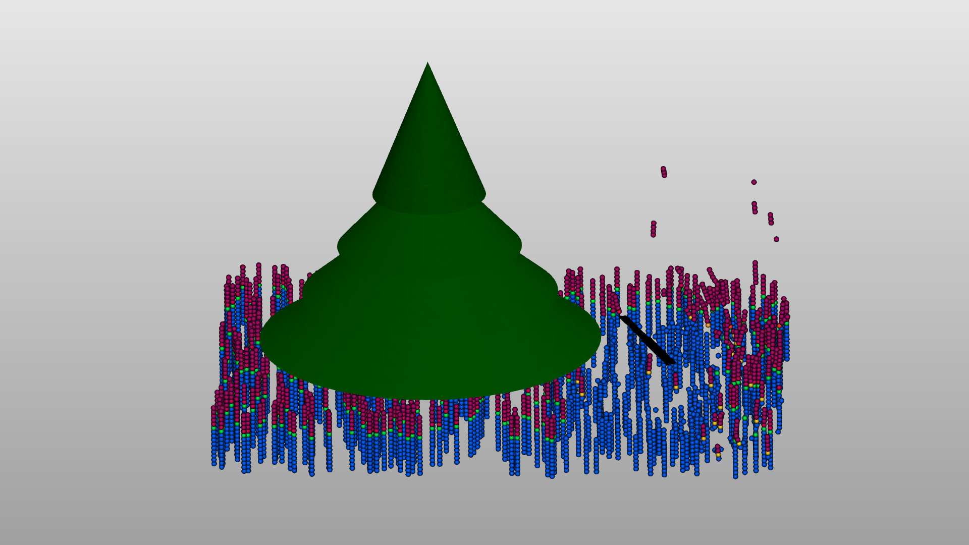
Name of the case: Project_Fibers

Setting up the Aspherix(R) GUI simulation

As a first step, the used materials command as well as the simulation domain are defined in the General Settings tab. Please note that in case of multiple dependent simulations, the dimensions of the simulation domain can only be defined in the first simulation. This means that the box forming the simulation domain has to be chosen big enough from the beginning.

General settings

In this simulation we set particles of particle shape fiber:

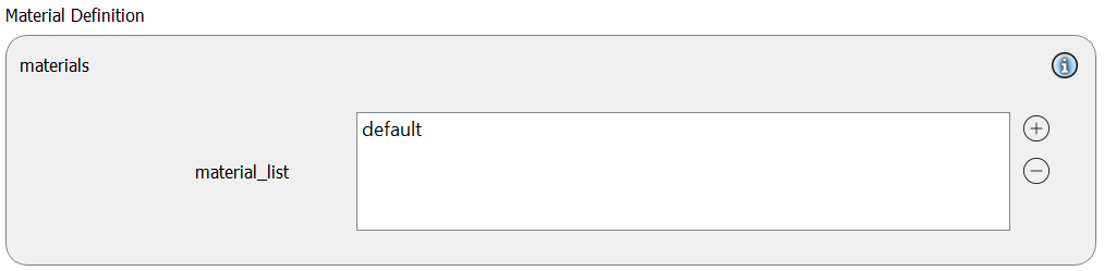
A single material named default is used:

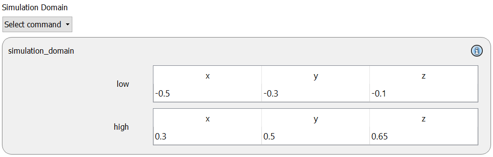
The simulation domain with x dimensions ranging from -0.5 to 0.3, y dimensions ranging from -0.3 to 0.5 and z dimension ranging from -0.1 to 0.65 is created:

Meshes and regions

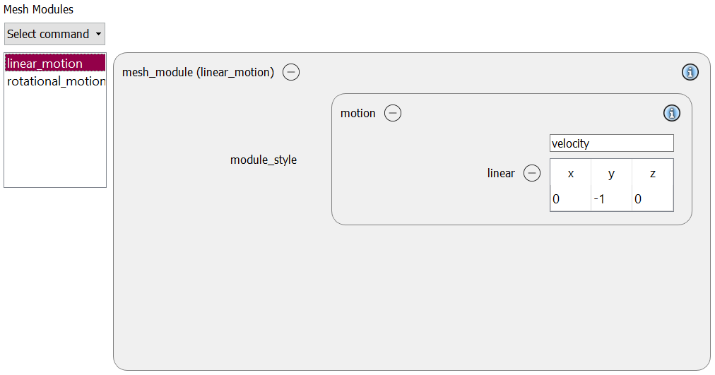
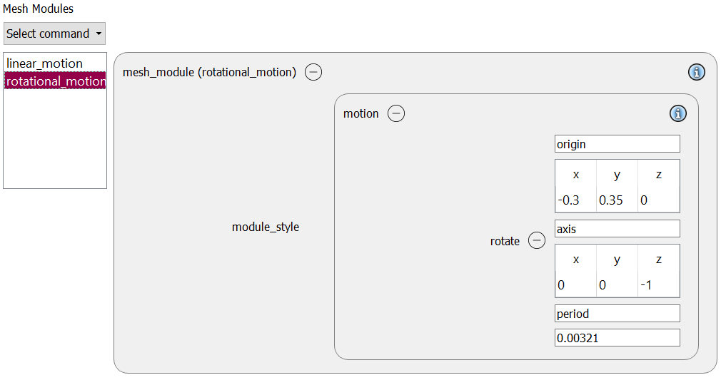
We start by creating two mesh modules of type motion for setting the rotational and translational blade motion:

Next, we load the geometry of the blade via the mesh command command:

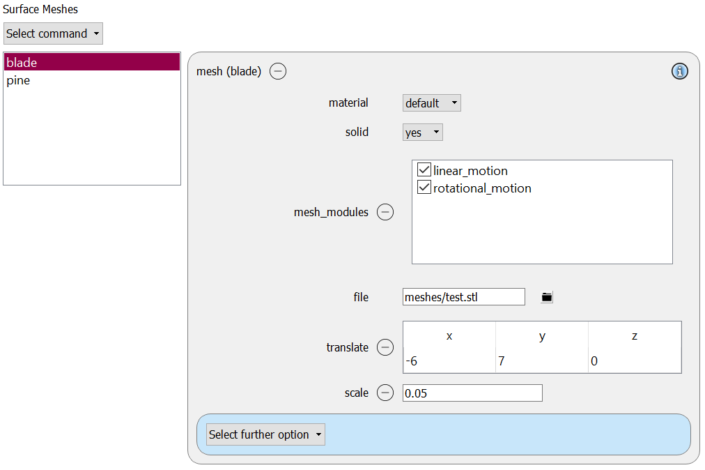
Please note that the two motion modules are added to the blade. The order in which the motion modules are applied is important and can be changed in the mesh_modules section of the mesh if required.

As an additional decoration, we add a second, pine-shaped mesh:

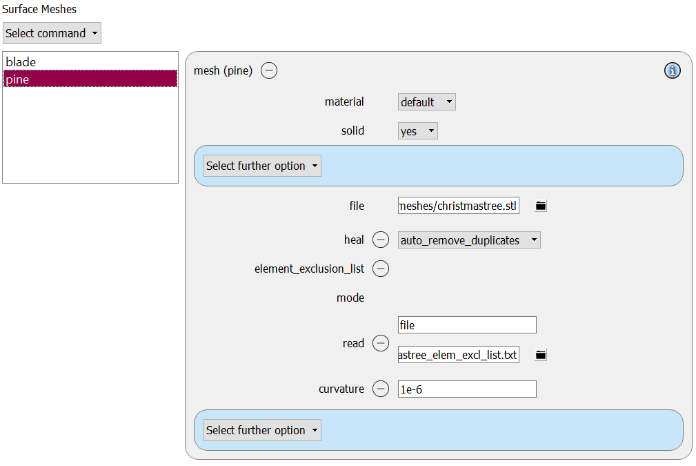
This mesh is more complex and has to be cleaned before using it. Please use the Mesh Healer tool (see Tools section of your Aspherix GUI) to create an element exclusion list. This element exclusion list is used as input to the element_exclusion_list command in read mode in this case. Furthermore the options heal auto_remove_duplicates and curvature 1e-6 are applied for a better mesh handling.

For the particle insertion a block-shaped region command called base_reg with the dimensions -0.5 to 0.3 in x, -0.3 to 0.3 in y and -0.0085500 to -0.0084500 in z dimension is defined:

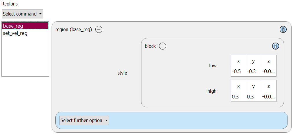
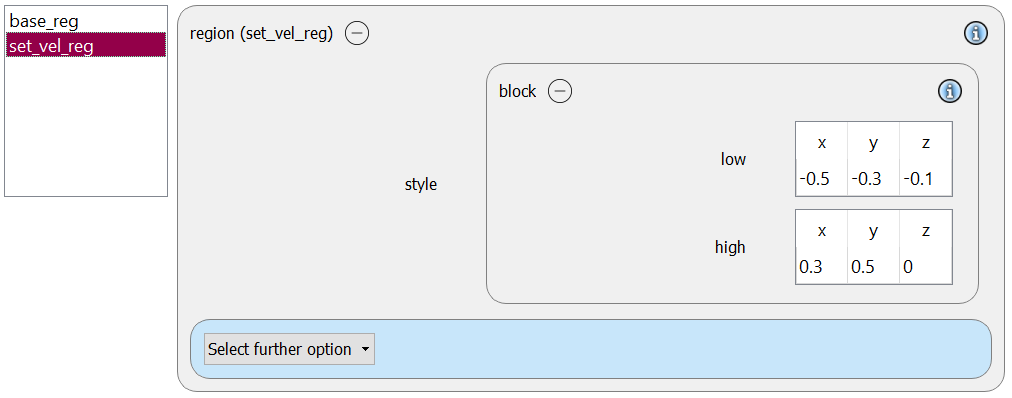
An additional region is created, in which we will later on set a constant velocity for all particles:

Physics models

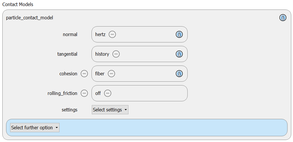
The contact models are now defined. For the particles we use the normal contact model hertz and the tangential model history. Since the particle shape in this simulation is set to fiber, it is mandatory to use the cohesion model fiber:

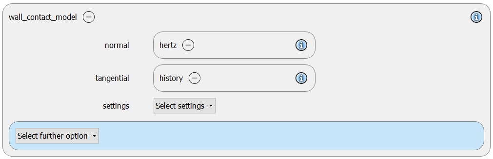
Since we added meshes in the previous section, a wall contact model is also added automatically to this section. We use the normal contact hertz and the tangential model history:

Finally, the gravity is enabled:

Per default the gravity has a magnitude of 9.807 and acts into negative z-direction. These defaults can be changed by either setting the magnitude or the direction manually.

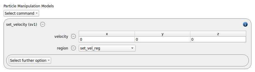
We use a set_velocity command command to set the velocity of the fibers in the region set_vel_reg to zero in all dimensions:

Particles

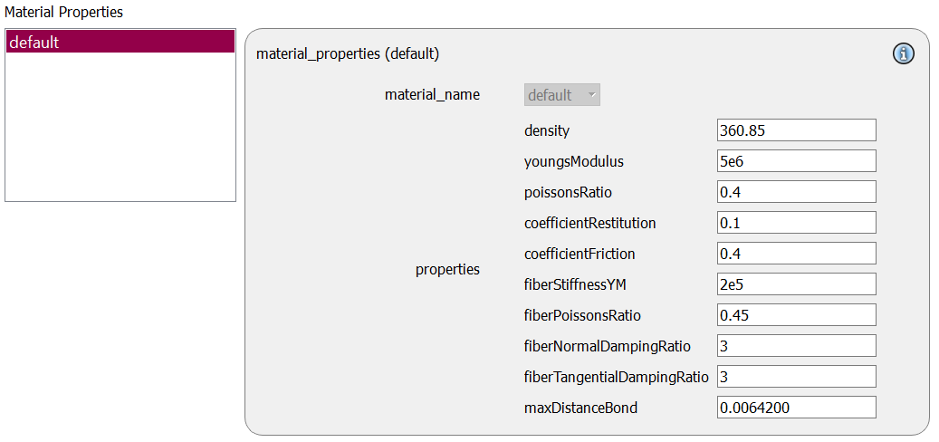
In the general settings tab we only defined a single material type (default), whose settings have to be specified here:

	default
Density	360.85
Young’s modulus	5e6
Poisson’s ratio	0.4
Coefficient of restitution	0.1
Coefficient of friction	0.4
fiberStiffnessYM	2e5
fiberPoissonsRatio	0.45
fiberNormalDampingRatio	3
fiberTangentialDampingRatio	3
maxDistanceBond	0.00642

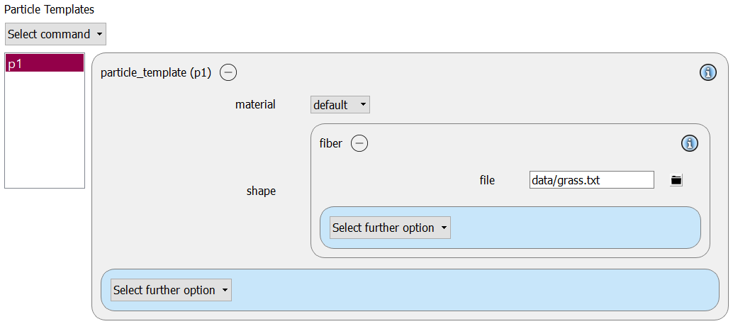
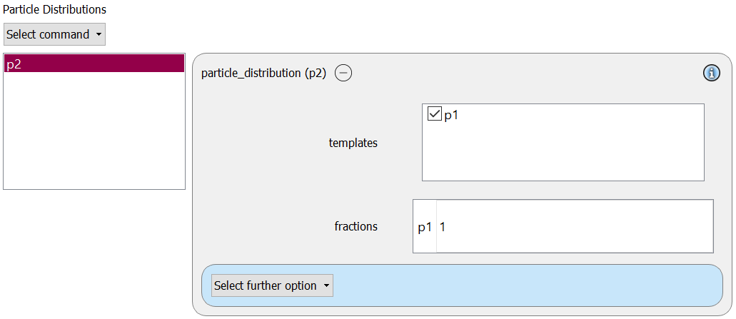
A particle template of shape fiber is generated from the input file data/grass.txt and used to form a particle distribution:

An insertion command of type pack is used to insert 534 particles with a velocity of 0.1 m/s in z-direction. They are inserted in the previously defined base_reg, and since the fibers are larger than the z-dimension of the region the keyword all_in is set to no.

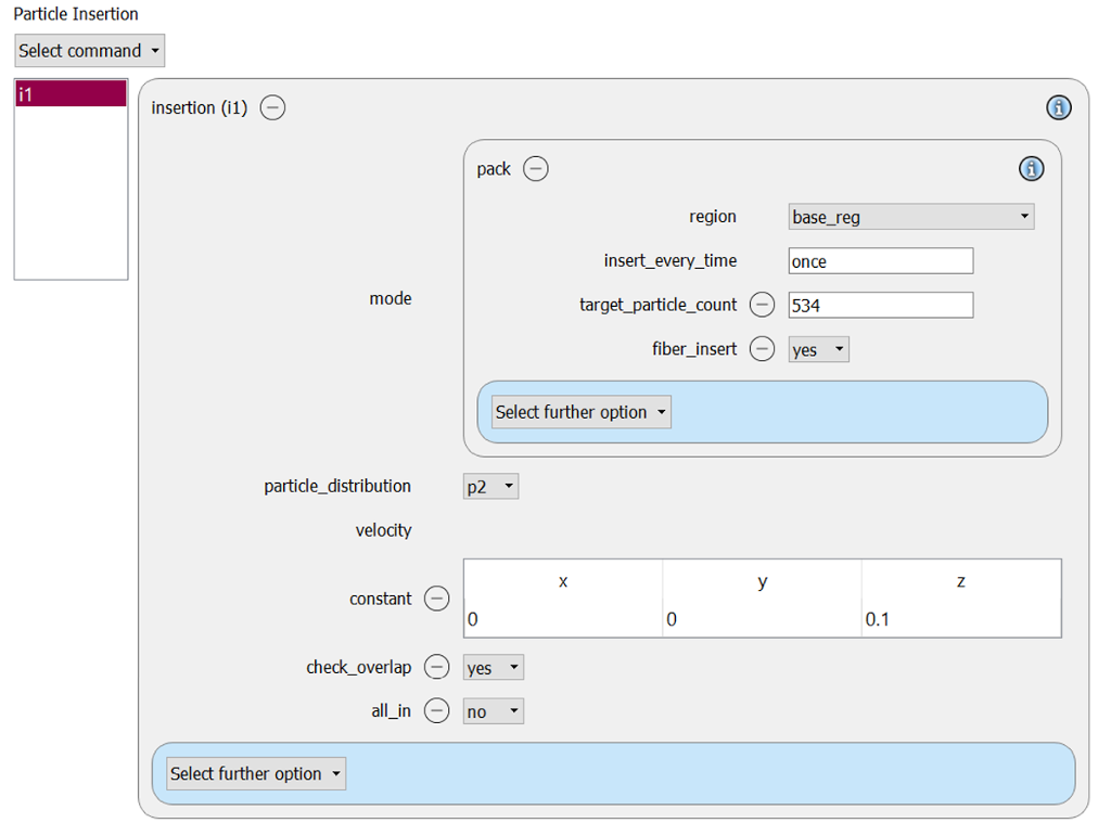
The insert_every_time is set to once, ensuring that the pack is inserted only once at the beginning.

Simulation control

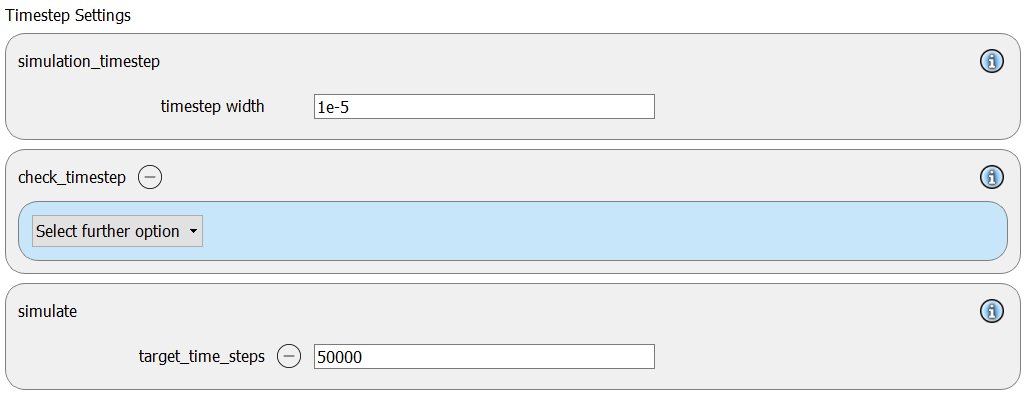
In this tab, we first define the time-step settings such as the desired simulation timestep of 1e-5 seconds and the total number of simulation time steps of 50000. Per default also the check_timestep command command is enabled, which throws a warning when the time step exceeds 10 % of the Rayleigh or the Hertz time. These thresholds can be changed by setting an alternative value for hertz_fraction or rayleigh_fraction.

Output settings

In this tab we first define the timestep width for the file and the terminal output:

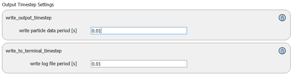
The “output_settings” command takes care that all particle information and the meshes are written to files. Furthermore, it triggers the output of global quantities such as the kinetic energy of the particles or total normal and shear stresses onto meshes in the terminal. Please note that if the output of per-cell information on meshes such as wear, velocity of stress are desired, one has to add the keyword mesh_properties and select the required output.

Running the simulation

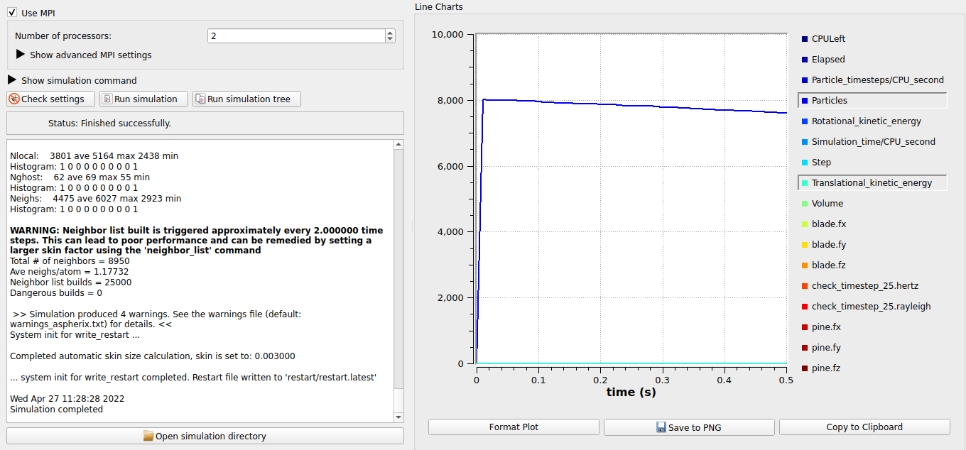
After completing the setup and saving it, the simulation can be launched. Hence, change to the Simulation view. First hit the “Check settings” button, and if the check returns “Check settings successfully completed” the simulation can be run by hitting “Start”. The graph shows the decay of the inital number of particles, since some of the cut grass is thrown out of the simulation domain.

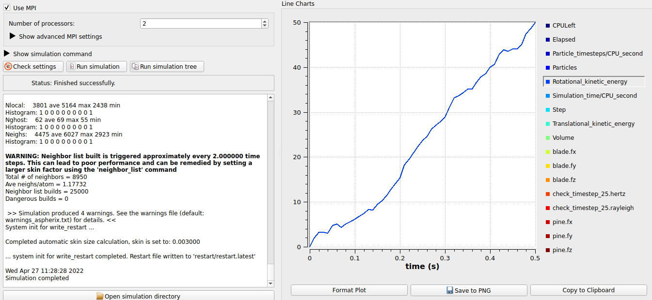
The impact of the blade causes the mowed grass to fly away, which is also indicated by an increase in the rotational kinetic energy:

Postprocessing with Paraview

After the simulation is completed, all data written with the output_settings command can be visualized automatically by going to the Visualization view and hitting the “Start Paraview” button.

The image shows the simulation after 45000 time steps. The grass is colored according to the z-position of the particles to emphasize that magenta tips are missing in the area through which the blade has already passed: