Flexible cubes (bonded particles)

In this tutorial we insert a group of cubes that consist of flexibly bonded spheres. In the course of the simulation the particles settle, forming a packing of deformed cubes in the end. This image shows the final state of the simulation (one the left: visualization of the particles; on the right: visualization of the bonds):

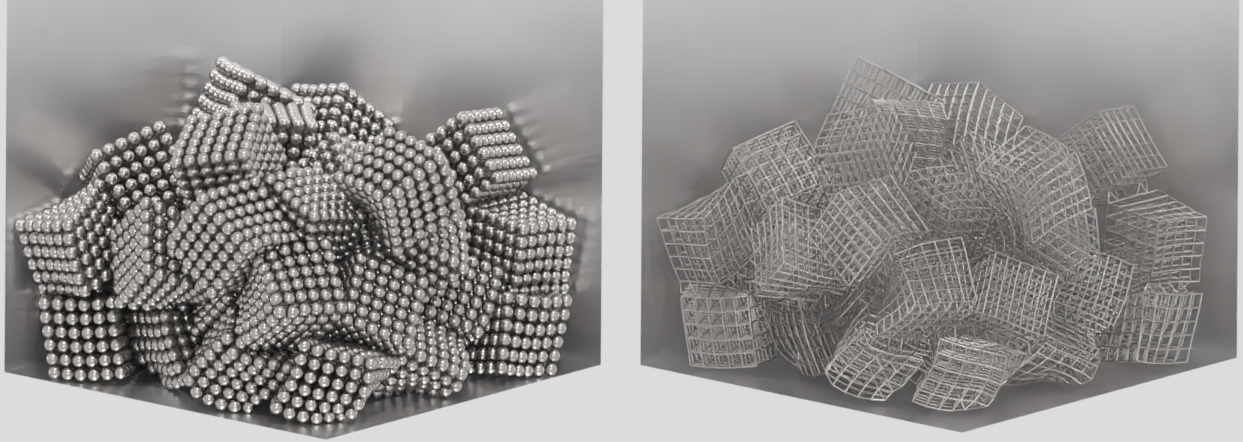
Name of the case: Project_Cubes_Bonded

Setting up the simulation

As a first step, the particle shape, the used material and the simulation domain are defined in the General Settings tab.

General settings

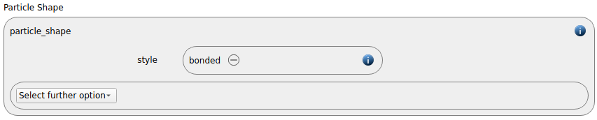
In this simulation we set particles of particle shape bonded:

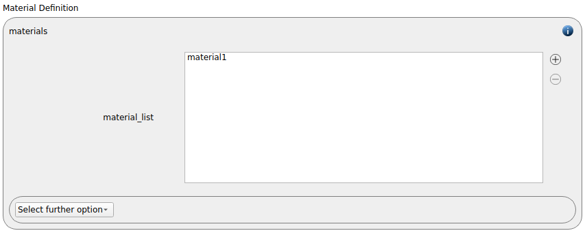
A single materials command with the name material1 is used:

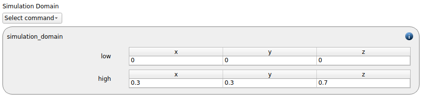
The simulation domain with x and y dimensions ranging from 0 to 0.3 and z dimensions ranging from 0 to 0.7 is created:

Meshes and regions

We use five primitive walls as domain boundaries:

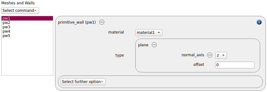
Type	Normal axis	Offset
plane	x	0
plane	x	0.3
plane	y	0
plane	y	0.3
plane	z	0

Physics models

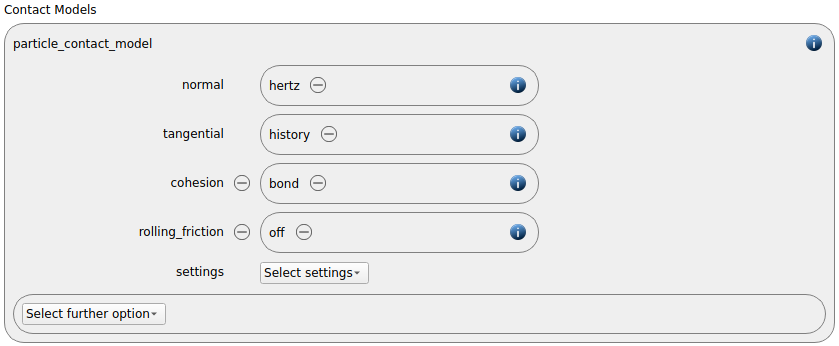
The contact models are now defined. For the particles we use the normal contact model hertz, the tangential model history and the cohesion model bond:

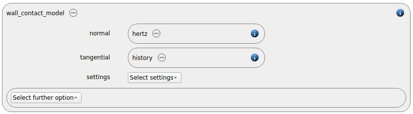
Since we added primitive walls in the previous section, a wall contact model is also added automatically to this section. We use the normal contact model hertz and the tangential model history:

The default gravity command is removed from the simulation setup.

Particles

In the general settings tab we only defined a single material type (default), whose settings have to be specified here:

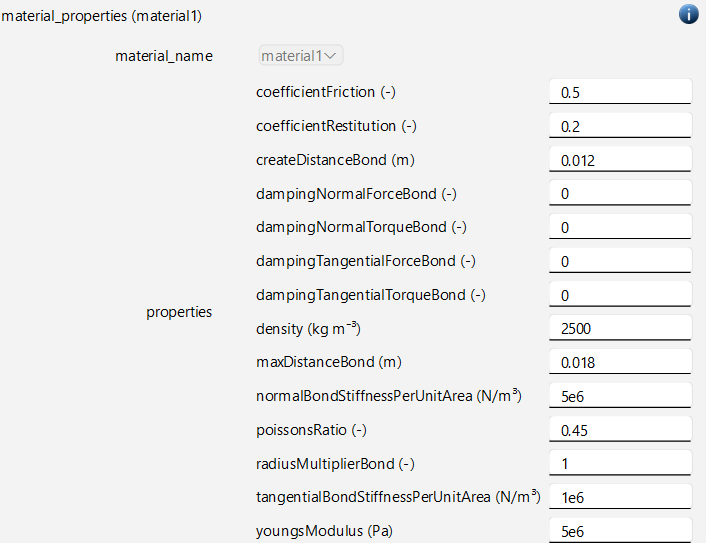
Please note that the list of properties contains more entries than actually required for the bond model in the used configuration. Other configurations that can be defined via adding keywords in the settings section require more input. Please set the values for the unnecessary parameters to zero (they will simply be ignored). Please have a look at the bond model documentation for more information.

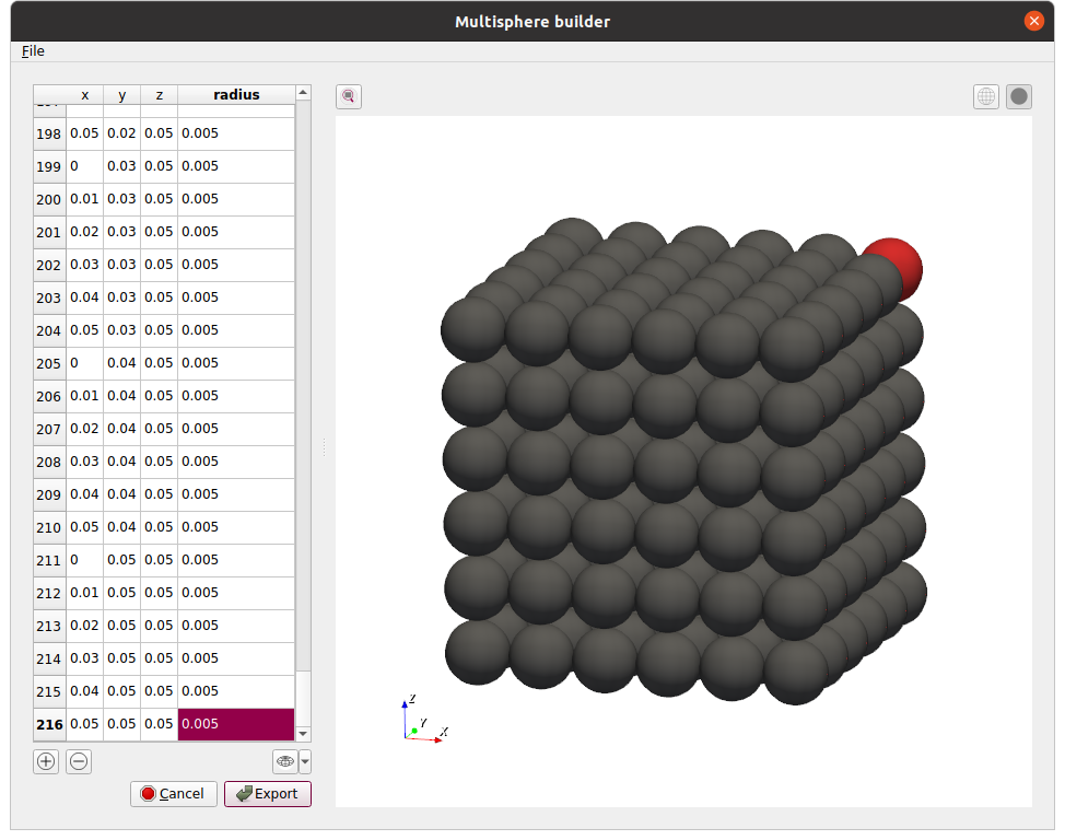
Particle templates for bonded particles use data files that consist of the list of spheres defined by radius and position (more information can be found here. These files can be generated manually, with scripts or by the multisphere builder. In the current case a particle consists of 216 sphere and looks as following when loaded in the multisphere builder (Tools/MS Builder):

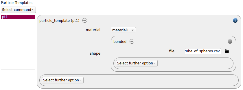
The generated particle file is used for a particle template of style bonded:

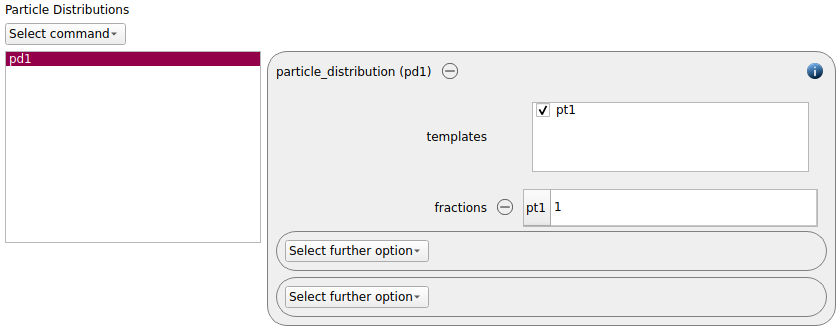
In the next step the particle distribution is generated:

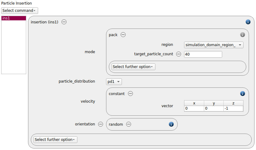
An insertion command command of type pack is defined with the following settings:

	insertion
mode	pack
region	simulation_domain_region_
target_particle_count	40
particle_distribution	pd1
velocity	constant (0,0,-1)
orientation	random

Simulation control

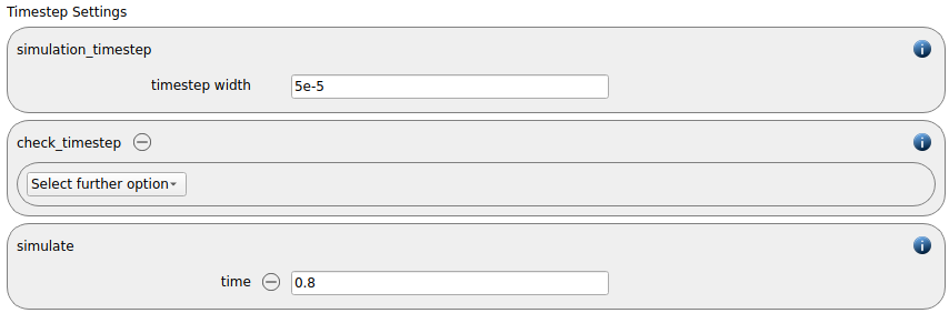
In this tab, we first define the time-step settings such as the desired simulation timestep of 5e-5 seconds and the total simulation time of 0.8 seconds. Per default also the check_timestep command command is enabled, which throws a warning when the time step exceeds 10 % of the Rayleigh or the Hertz time.

The enable_loadbalancing command command is added by default and ensures an optimal usage of the computational resources when running the case in parallel:

Output settings

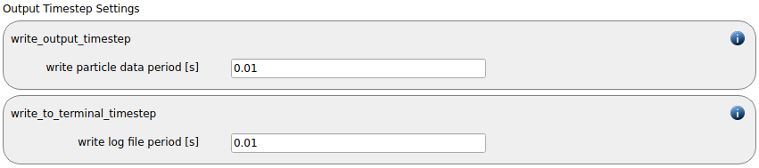
In this tab we first define the timestep width for the file and the terminal output:

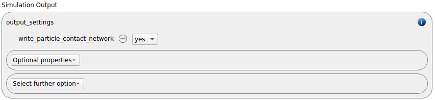
The output_settings command command the takes care that all particle information and the meshes are written to files accordingly. The option write_particle_contact_network is set to yes, so also the particle-particle contacts plus the according forces can be visualuized:

Running the simulation

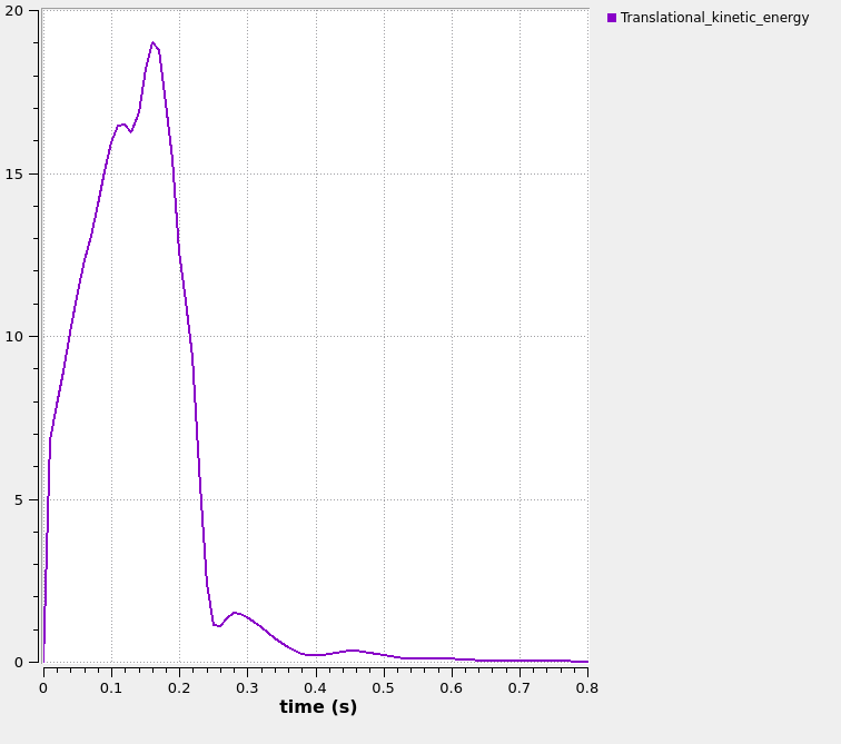
After completing the setup and saving it, the simulation can be launched in the “Simulation” tab. For the given number of particles (in terms of sub-spheres) a parallel calculation on two cores is a good choice. The graph shows the kinetic energy of the system after the simulation run is completed:

Postprocessing with Paraview

After the simulation is completed, all data written with the output_settings command can be visualized automatically by going to the Visualization view and hitting the “Start Paraview” button.

This image shows the final state of the simulation (one the left: visualization of the particles; on the right: visualization of the bonds):