Output particles with overlay meshes

This tutorial shows how to replace particles with overlay meshes in the output. In two examples, multispheres and superquadrics are replaced.

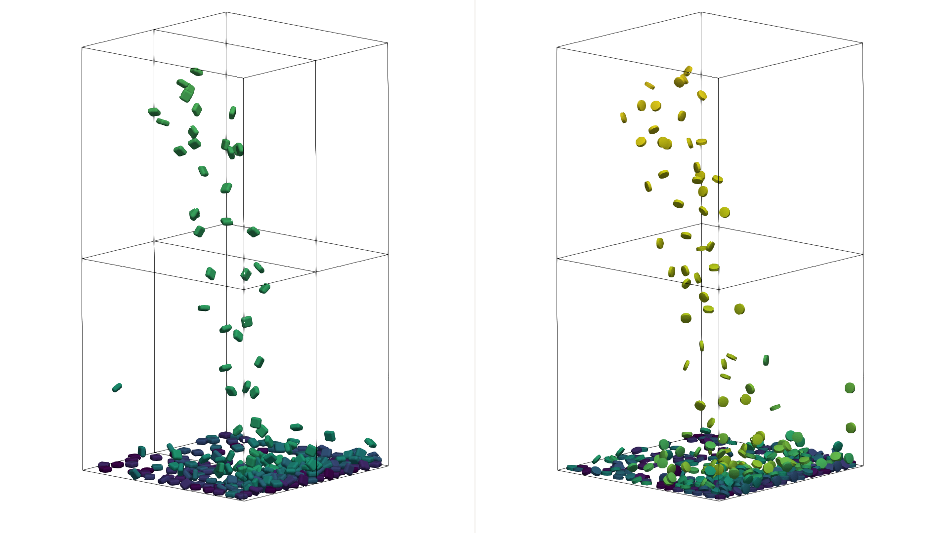
The image shows the final result of the multisphere (left) and superquadric (right) case. In both cases the original particles are replaced by mesh files in the output. During the calculation the original particle shapes are used for the contact detection.

Name of the case: Project_Meshed_Particle_Overlay

Case 1: Superquadric Case

As a first step, the particle shape, the used materials command and the simulation domain are defined in the General Settings tab.

General settings

In this simulation we set particles of particle shape sphere:

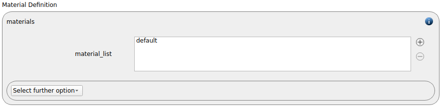
A single material called “default” is used for walls and particles:

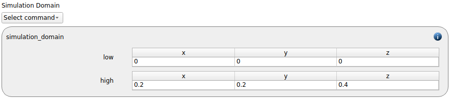
The simulation domain ranging from 0 to 0.2 in x, from 0 to 0.2 in y and from 0 to 0.4 in z direction is created:

Meshes and regions

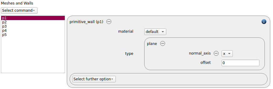
Five primitive walls are used as solid walls for the simulation domain:

name	type	normal_axis	offset
p1	plane	x	0
p2	plane	x	0.2
p3	plane	y	0
p4	plane	y	0.2
p5	plane	z	0

Physics models

The contact models are now defined. For the particles we use the normal contact model hertz and the tangential model history.

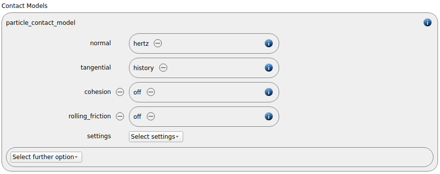
Since this is a very basic test case, the gravity is removed.

Particles

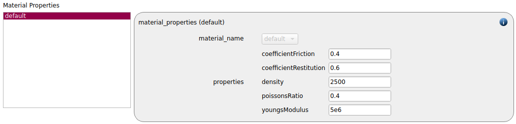
In the general settings tab the material properties are defined:

	default
Density	2500
Young’s modulus	5e6
Poisson’s ratio	0.4
Coefficient of restitution	0.6
Coefficient of friction	0.4

Next, we open the superquadric builder to generate a superquadric object for the particle template. It can either be accessed through the button in the symbol bar or through Tools / Non-spherical particles / Superquadric Builder.

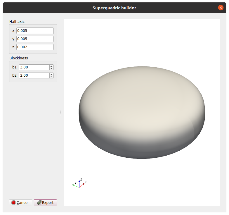
We chose (0.005, 0.005, 0.002) for the half-axis and (3,2) for the blockiness. By pressing the “Export” button the shape is automatically exported to a particle template.

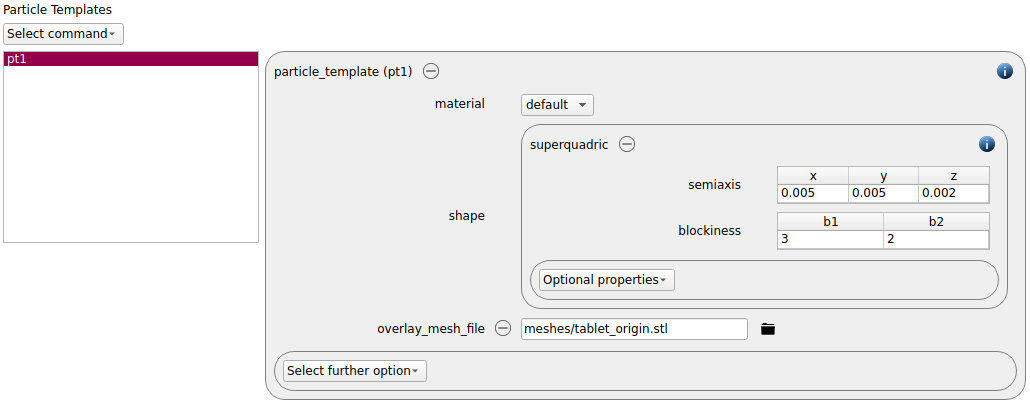
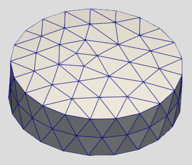
For the planned mesh overlay the keyword overlay_mesh must be defined. We use this prepared mesh:

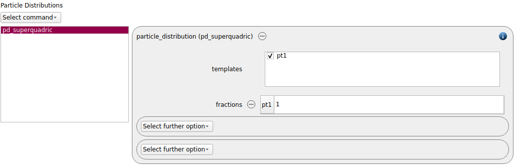
Then, a particle distribution is created.

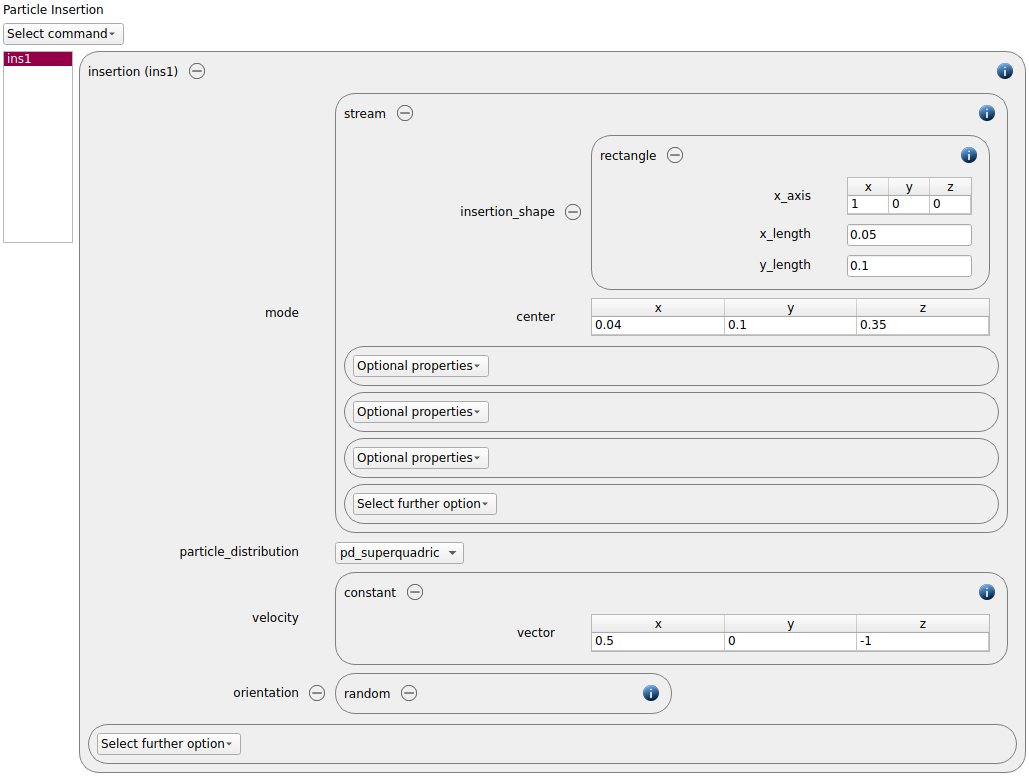
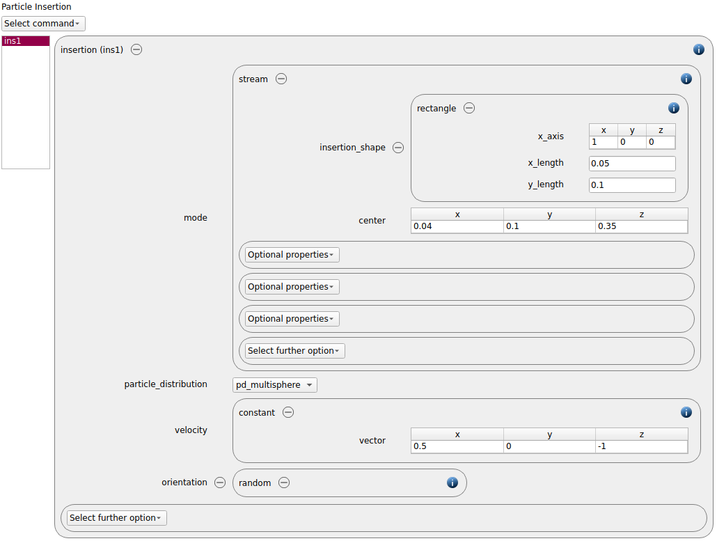
An insertion command command of type steam is used. InWe use a rectangular insertion face to insert the particles with a velocity of (0.5,0,-1) m/s. The particle orientation is set to random.

Simulation control

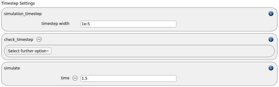
In this tab, we first define the time-step settings such as the desired simulation timestep of 1e-5 seconds and the total simulation time of 1.5 seconds. Per default also the check_timestep command command is enabled, which throws a warning when the time step exceeds 10 % of the Rayleigh or the Hertz time. These thresholds can be changed by setting an alternative value for hertz_fraction or rayleigh_fraction.

Loadbalancing is enabled per default:

Output settings

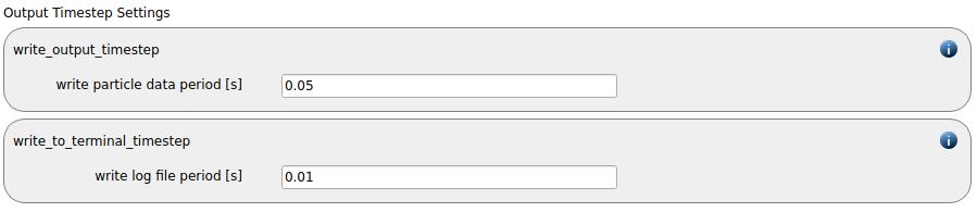
In this tab we first define the timestep width for the file and the terminal output:

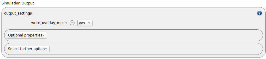
The output_settings command command the takes care that all particle information is written to files accordingly. Furthermore it triggers the output of global quantities such as the kinetic energy of the particles to the terminal. For replacing the particles by their overlay meshes in the output, we add the keyword write_overlay_mesh:

Running the simulation

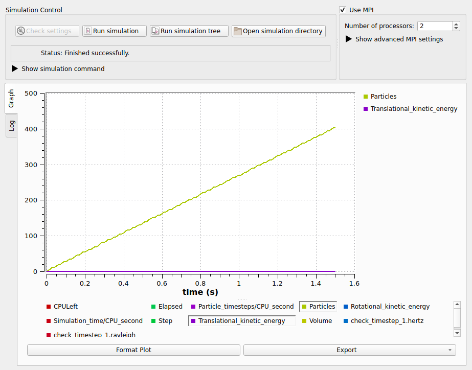
After completing the setup and saving it, the simulation can be launched. Change to the Simulation view and set the number of cores to use to 2.

Postprocessing with Paraview

After the simulation is completed, all data written with the output_settings command can be visualized automatically by going to the Visualization view and hitting the “Start Paraview” button.

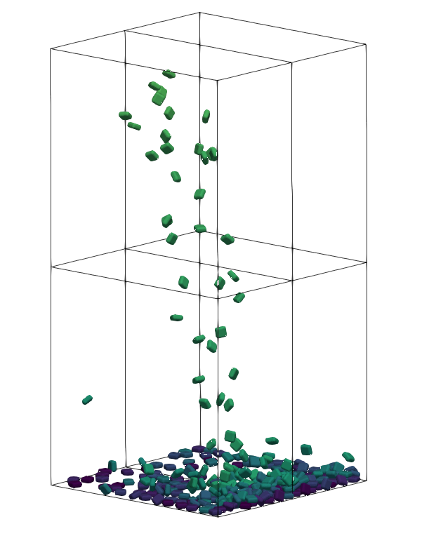
The image below shows the final state of the system:

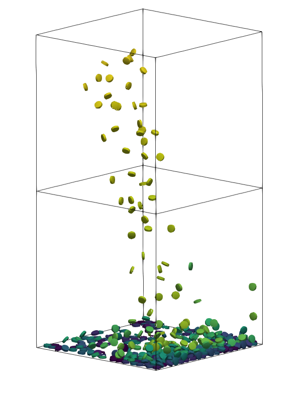
The image shows the state of the simulation at the last time step, the particles are colored by id. The particles are represented by their overlay meshes, this result can be used for further postprocessing. Please note that the default output is binary, but it can be changed to ascii by adding this keyword to the output_settings command.

Case 2: Multisphere Case

For applying this functionality for multispheres, only few adaptions are required. We therefore start by cloning the previous simulation.

General settings

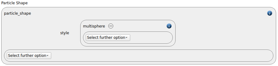
Then, we go to the General Settings tab and change the particle shape from superquadric to multisphere:

Particles

All other changes required are made in the Particles tab.

We first start with the generation of the multisphere particle. This can be done with the help of the multisphere builder, which accessed through the button in the symbol bar or through Tools / Non-spherical particles / Multisphere Builder. Alternatively, the multisphere file can also be generated otherwise (e.g., with the help of a script or excel / libre office, in case more spheres are present) and then be visualized through the Multisphere builder:

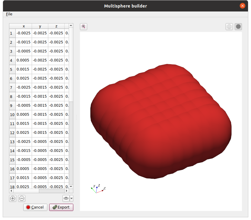
By pressing the export button, the multisphere data file is saved to the data folder of the case and added to a particle template.

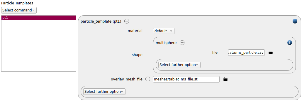
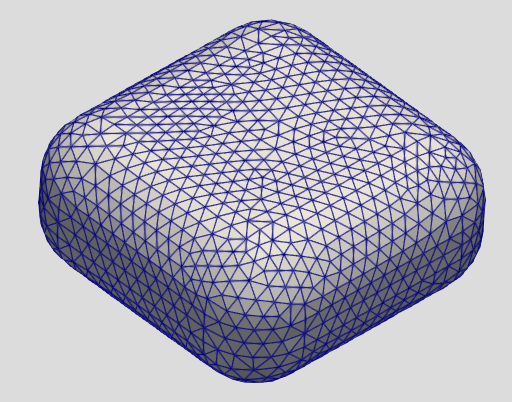
Just as previously for the superaudric we use the keyword overlay_mesh_file to define the mesh that will replace the multispheres in the output. This is the mesh that is used in that case:

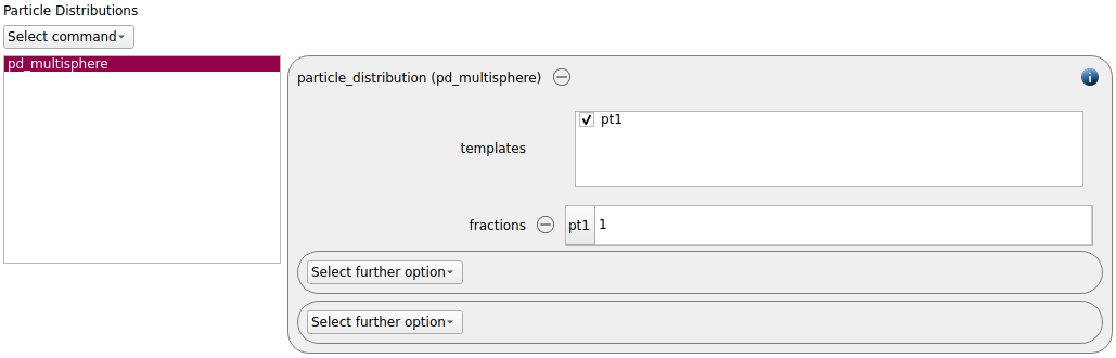
The particle template is then used in a particle distribution, which is then used for the insertion command:

These were the last changes required, the case can now be saved.

Running the simulation

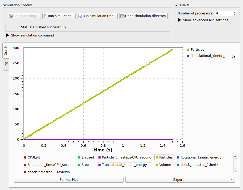
Since the multispheres consist of a remarkable number of spheres in this case, using 4 instead of 2 cores brings increased simulation speed:

Postprocessing with Paraview

After the simulation is completed, all data written with the output_settings command can be visualized automatically by going to the Visualization view and hitting the “Start Paraview” button.

The image below shows the final state of the system: