Automatic workflow for filling complex regions with spheres

In this case we show how to set up an automated workflow for filling a complex region with a dense packing of spheres. Instead of defining a specific simulation time we use the simulate command in mode “until_filled”. In this mode the simulation runs until the mass in a defined region does not change any more.

A dense packing algorithm for spherical particles is used to create a possibily dense intial packing and thus to speed up the filling process.

Name of the case: Project_Packing_Generation_Spheres

Simulation Setup: Filling the region

In this simulation we insert a possibly dense packing of spheres in the target region. A second insertion command is used that starts adding more particles. The simulate command in mode “until_settled” triggers the simulation to run until the mass in the target region becomes constant.

We start with generating a new project and adding a new simulation to it:

General settings

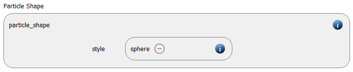
In this simulation we use particles of particle_shape command sphere:

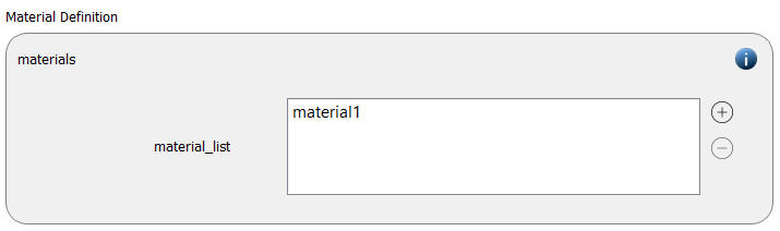
A material with name material1 is defined:

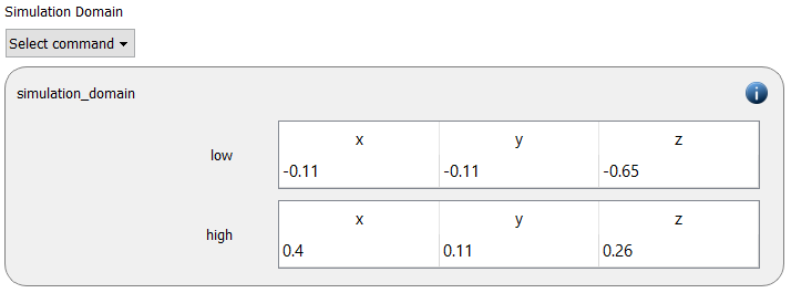
The simulation domain is defined with x-dimensions ranging from -0.11 to 0.4, y-dimensions ranging from -0.11 to 0.11 and z-dimensions ranging from -0.65 to 0.26 meters:

Meshes and regions

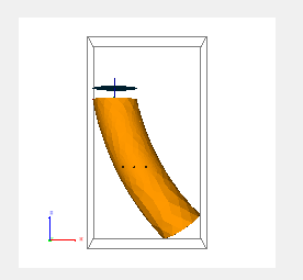
Altogether this simulation involves 3 meshes: one mesh command forms the walls of the region, one is used to close it at the bottom and a third component is used as insertion face for the continuous particle stream:

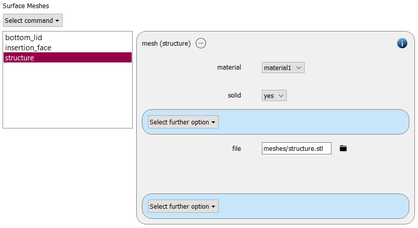
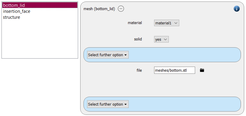
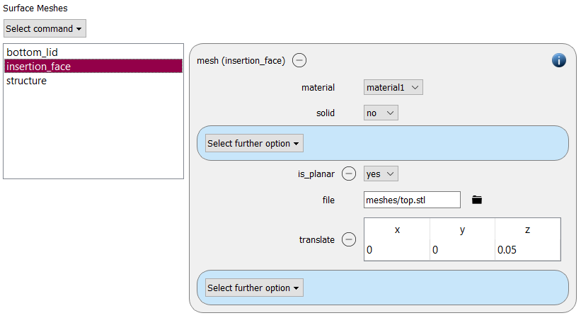
After loading the mesh files they are visualized in the graphical preview window:

For the particle insertion later on we require an insertion region of style mesh/vtk:

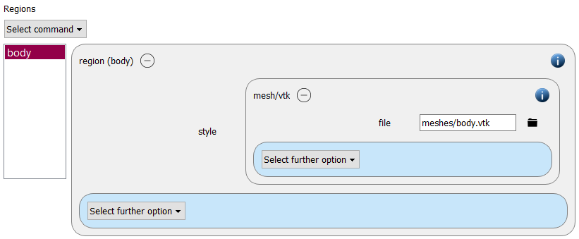
Hint: meshes that are used for generating regions must be 3D vtk meshes. Example for obtaining such a mesh file: when exporting meshes in GMF format (ending: .mesh) from Salome, the tool Gmsh can be used to convert them to .vtk.

Physics models

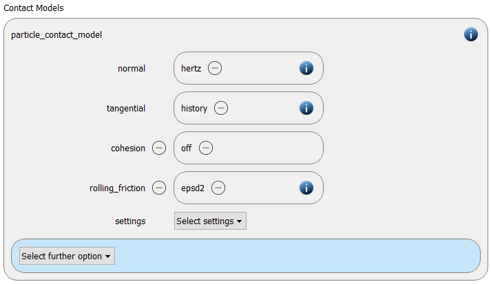
In the next step, the definition of the physics models takes place. For the particles we use the normal contact model hertz, the tangential model history and the rolling friction model epsd2.

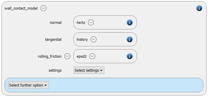
Since we added meshes in the previous section, also a wall contact model was added automatically in this section. We use the same contact models as for the particles:

Finally also the gravity is defined:

Per default the gravity has a magnitude of 9.807 and acts into negative z-direction. These defaults can be changed by either setting the magnitude or the direction manually.

Particles

In the general settings tab we introduced two materials. Here we define the required material properties.

	material1
Density	2000
Young’s modulus	5e6
Poisson ratio	0.43
Coefficient of restitution	0.3
Coefficient of friction	0.5
Coefficient of rolling friction	0.05

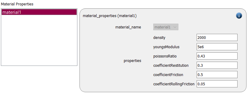
In the next step three particle templates with a radius of 0.004, 0.005 and 0.006 meters respectively are generated:

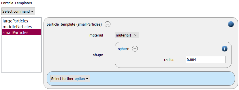
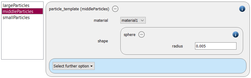
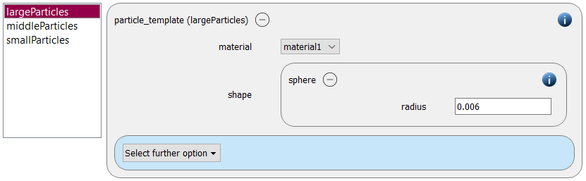
These three templates are used to define a particle distribution:

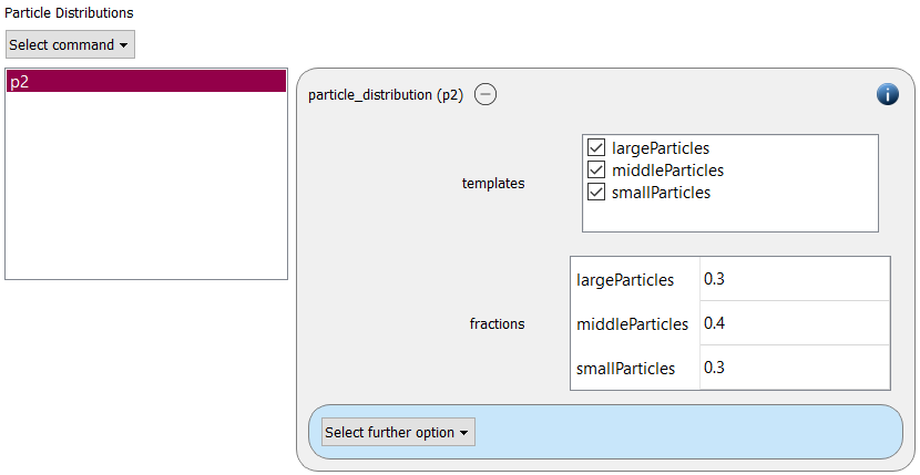
An insertion command in mode pack is used for particle insertion. Please note that the target volume fraction is set to 0.8, which is a very high value for the standard particle insertion algorithm. Typically, this value cannot be reached, and this could lead to a mis-representation of the particle distribution. We therefore use the packing_generator of style dense. This algorithm is on the one hand able to insert much denser particle packings, and on the other hand the correct particle distribution is maintained, even when the desired packing density cannot be achieved:

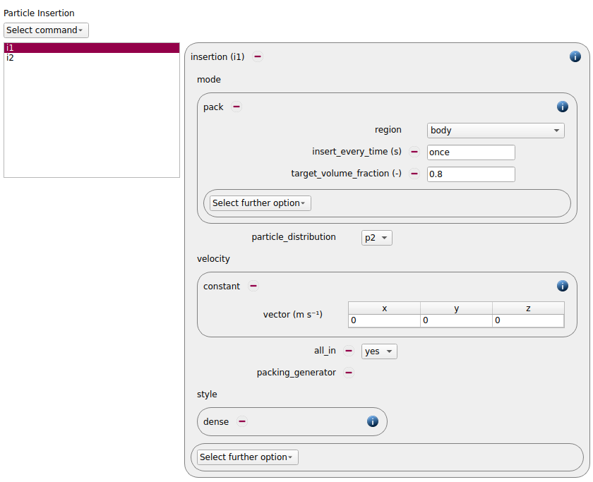
Using a volume fraction of 0.8 will lead to a warning (with the given particle distribution such a high packing density is impossible - even theoretically) but it ensures that as many particles are inserted as somehow possible.

Since some more particles will be needed for a full dense packing (some settling will take place) we add another insertion command of type stream:

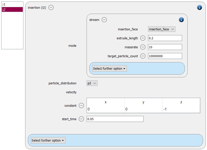
Simulation control

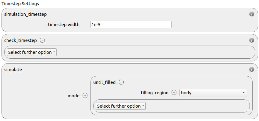
In this tab one first choses the time step settings such as the desired simulation timestep of 1.e-5 seconds. The simulate command command is used in mode “until_filled”, as filling region we use the region “body”.

Per default also the check_timestep command command is enabled, which throws a warning when the time step exceeds 10 % of the Rayleigh or the Hertz timestep. These thresholds can be changed by setting an alternative value for hertz_fraction or rayleigh_fraction.

Output settings

In this tab we first define the timestep width for the file and the terminal output:

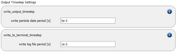
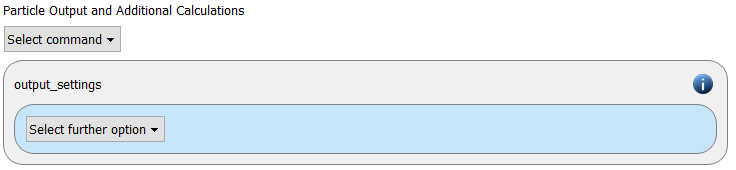
The output_settings command command takes care that all particle information and the meshes are written to files accordingly. Furthermore it triggers the output of global quantities such as the kinetic energy of the particles or total normal and shear stresses onto meshes in the terminal. Please note that if the output of per-cell information on meshes such as wear, velocity or stress are desired, the keyword mesh_properties has to be added and the required output has to be selected.

Running the filling simulation

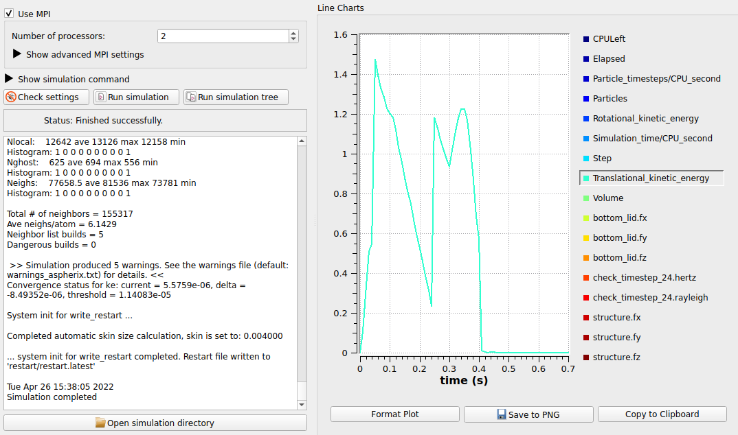
After saving the case we can change to the Simulation section. By hitting the Start button we can start running the simulation either serially or in parallel, using mpi. The loop script provides data for the number of particles, the kinetic energy, the total mass in the region and the kinetic energy in the region. The graph below (mass in the region) shows the kinetic energy during the filling process: whenever a new pack of particles is inserted it rises, after the last insertion it drops and approaches zero.

Result

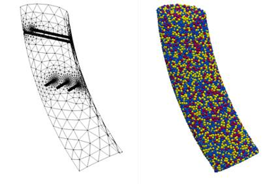
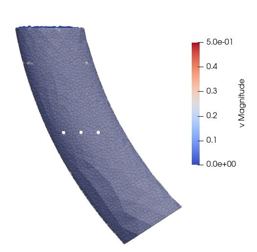
The result of the calculation can then be visualized with Paraview. The image shows the state of the particle bed at the end of the simulation:

Name of the case: Project_Packing_Generation_Spheres