Laser simulation with DEM

This tutorial shows the simulation of a laser beam reflected by a mirror on a particles bed. It is divided in two steps, in the first simulation we create the particle bed, while in the second we add the laser and the mirror.

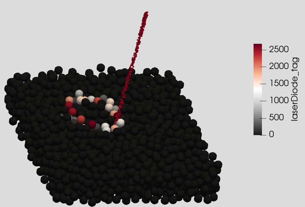
The image shows the particles bed colored with the laser tag value.

Name of the case: Project_Laser

Insertion

As a first step, the particle shape, the used materials command and the simulation domain are defined in the General Settings tab.

General settings

In this simulation we set particles of particle shape sphere:

Two regular materials command “particleMaterial” and “wallMaterial” and a single custom material “laser” are generated:

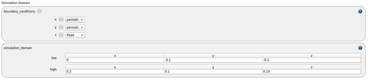
The simulation domain ranging from 0 to 0.2 in x, from -0.1 to 0.1 in y and from -0.1 to 0.15 in z direction is created and periodicity in x and y direction is imposed:

Meshes and regions

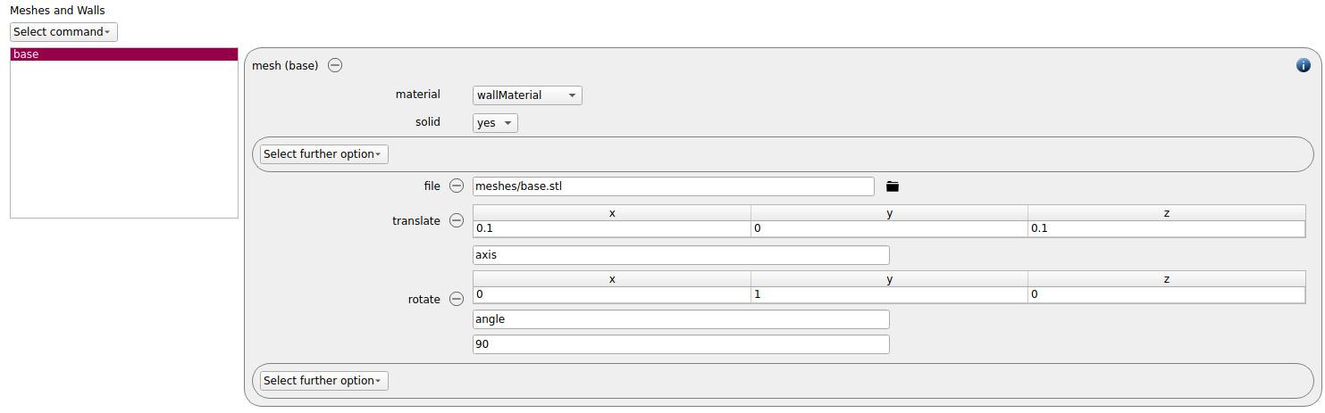
For the baseplate, a mesh command is inserted. We use a stl file and we rotate and translate it in the desired position.

Physics models

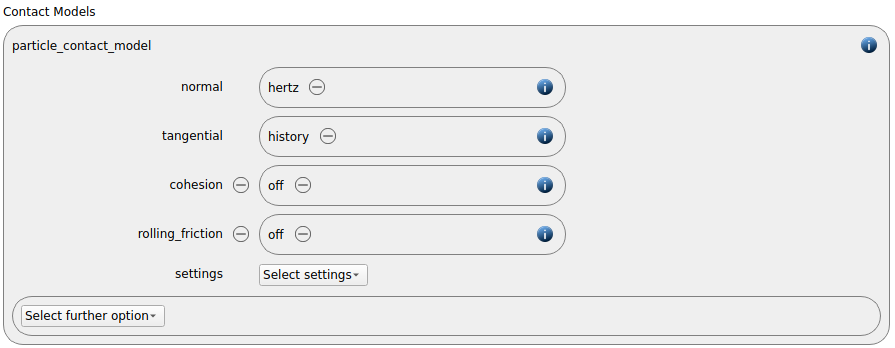
The contact models are now defined. For the particles we use the normal contact model hertz and the tangential model history.

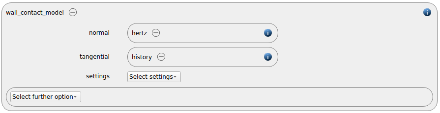
Since we added a mesh in the previous section, a wall contact model is also added automatically to this section. We use the default models normal hertz and tangential history:

We also enable heat transfer :

and the gravity :

Particles

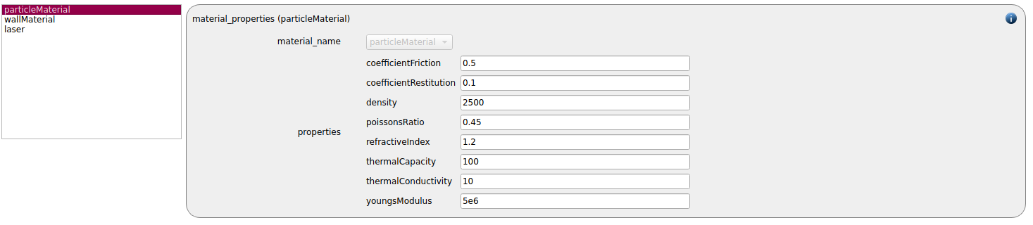
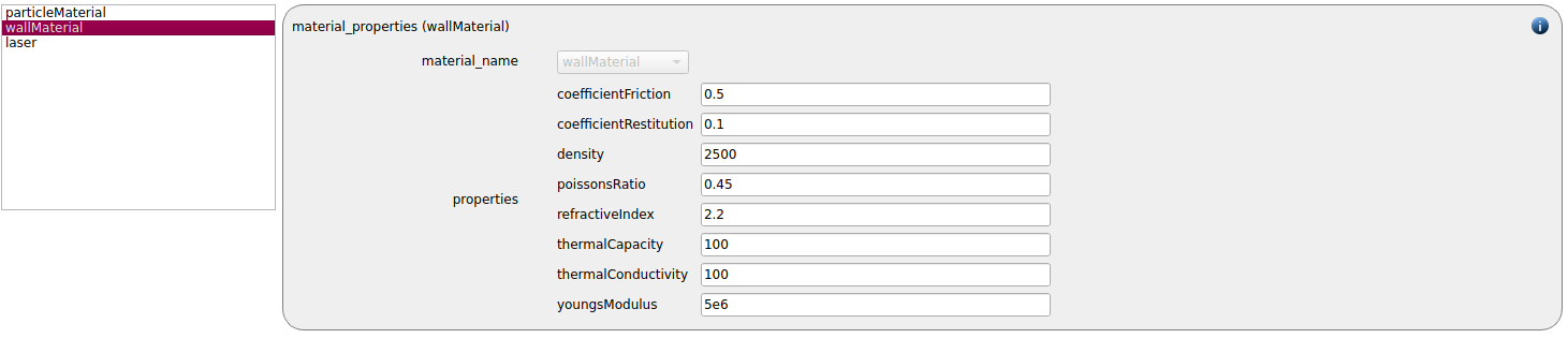
In the general settings tab the material properties for the particle_material and the wall_material are specified:

	particleMaterial	wallMaterial
Density	2500	2500
Young’s modulus	5e6	5e6
Poisson’s ratio	0.45	0.45
Coefficient of restitution	0.1	0.1
Coefficient of friction	0.5	0.5
Refractive index	1.2	2.2
Thermal capacity	100	100
Thermal conductivity	10	100

For the laser, the custom material properties are required:

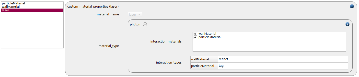
In this case, the laser particles will be reflected by the wall, and they will tag particles when they hit them.

Since two solid materials are present, also the material interaction properties must be set:

	wall_material - particle_material
Coefficient of friction	0.5
Coefficient of restitution	0.1

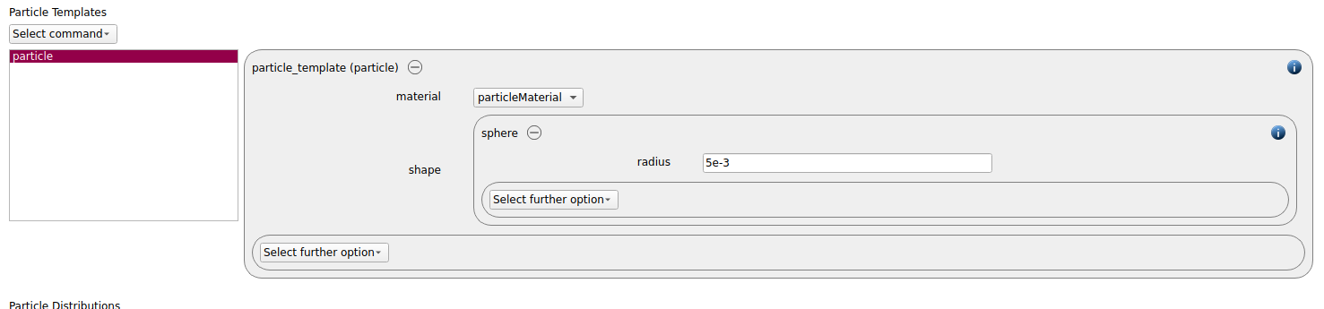
For the particles bed, one particle template of shape sphere with radius of 0.005 is added:

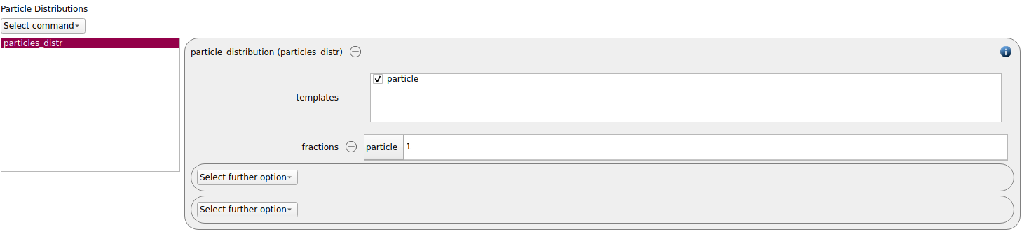
We also add the particle distributions:

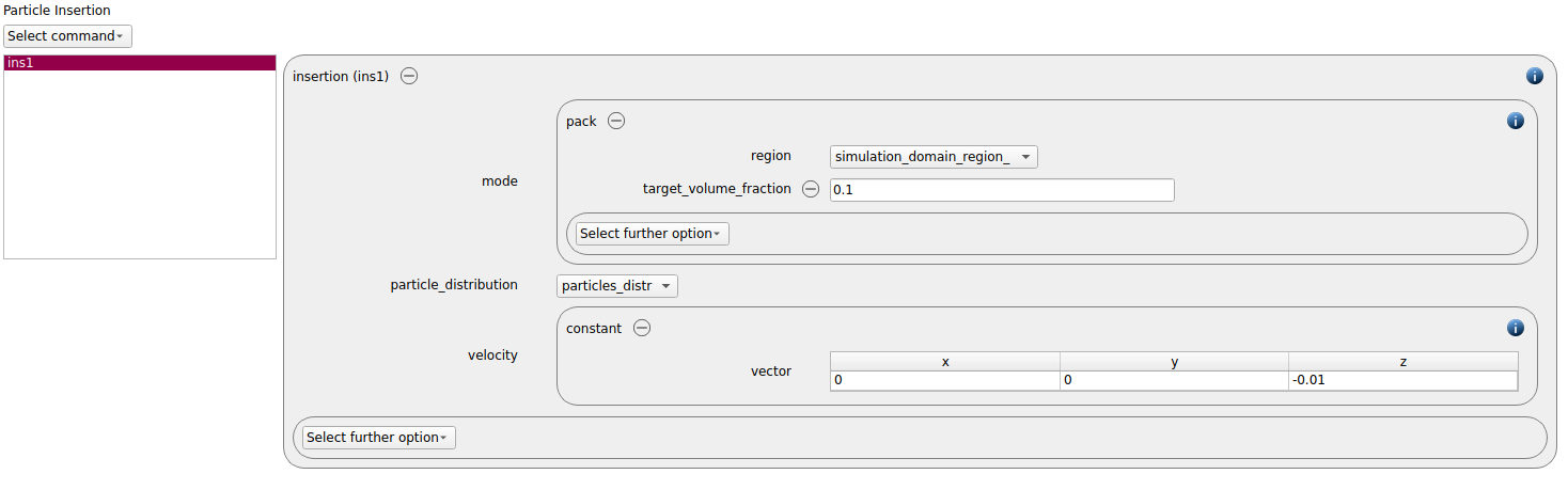
To create the particles bed we use a pack insertion command, using the whole domain as insertion region. The insertion velocity is -0.01 m/s in negative z-direction and the target volume fraction is 0.1 :

Simulation control

In this tab, we first define the time-step settings such as the desired simulation timestep of 9e-5 seconds and the total simulation time of 1 second. Per default also the check_timestep command command is enabled, which throws a warning when the time step exceeds 10 % of the Rayleigh or the Hertz time. These thresholds can be changed by setting an alternative value for hertz_fraction or rayleigh_fraction.

Output settings

In this tab we first define the timestep width for the file and the terminal output:

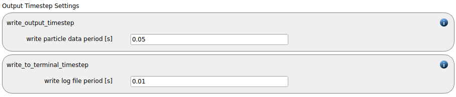
The output_settings command command the takes care that all particle information and the meshes are written to files accordingly. Furthermore it triggers the output of global quantities such as the kinetic energy of the particles or total normal and shear stresses onto meshes to the terminal. Please note that if the output of per-cell information on meshes such as wear, velocity of stress are desired, one has to add the keyword mesh_properties and select the required output.

Running the simulation

After completing the setup and saving it, the simulation can be launched by hitting “Run simulation”.

Laser

The second step, require us to set up the laser properties. The easy way is to use the “Clone simulation” command, clone the previous simulation and add the command needed to simulate the laser.

Meshes and regions

We have to add a mesh which act as a mirror for the laser. For the mesh command, we use the same stl file we used in the previous only scaled and translated.

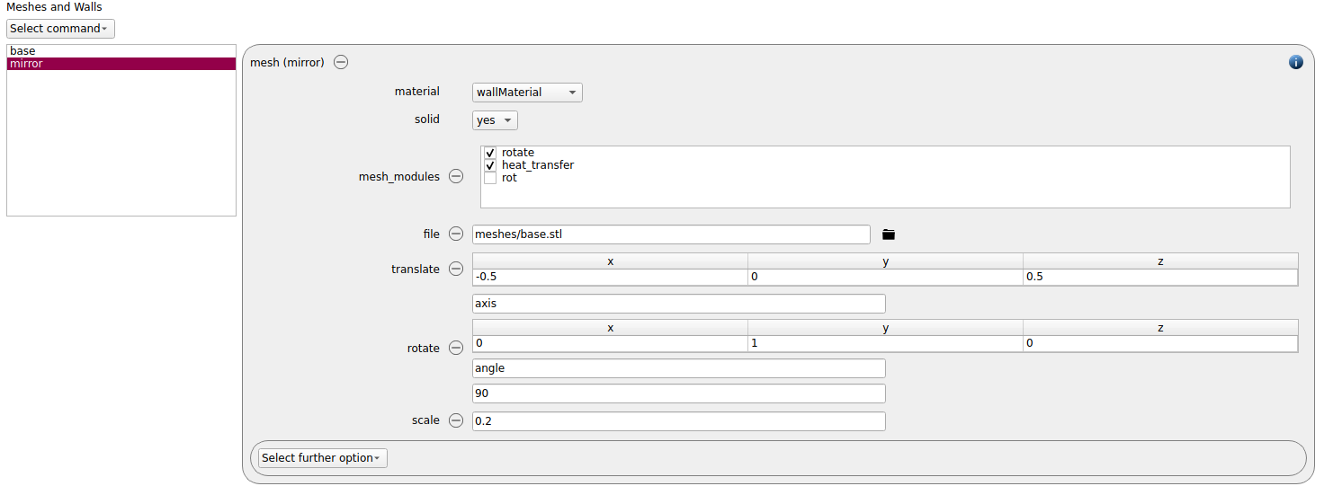
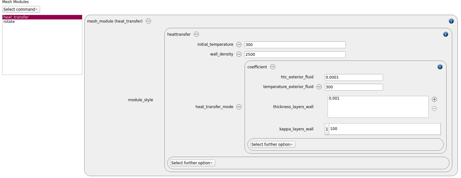
Note that we also add two mesh modules, heat transfer.

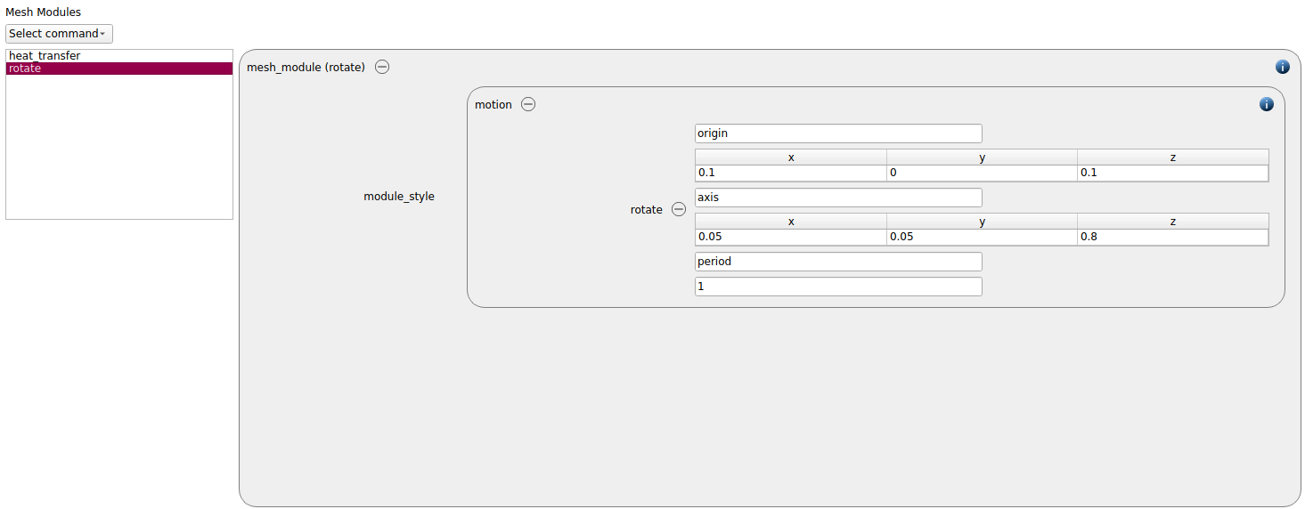
and rotate

Particles

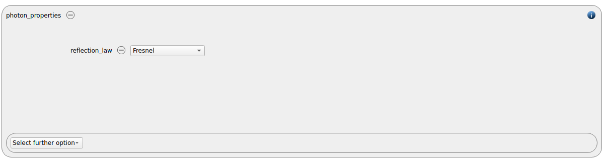
In the material properties, we have to add the photon properties:

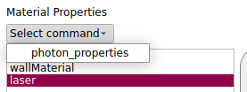
and we choose the Fresnel reflection law

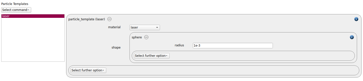
We add a particle template of shape sphere with radius of 0.001 :

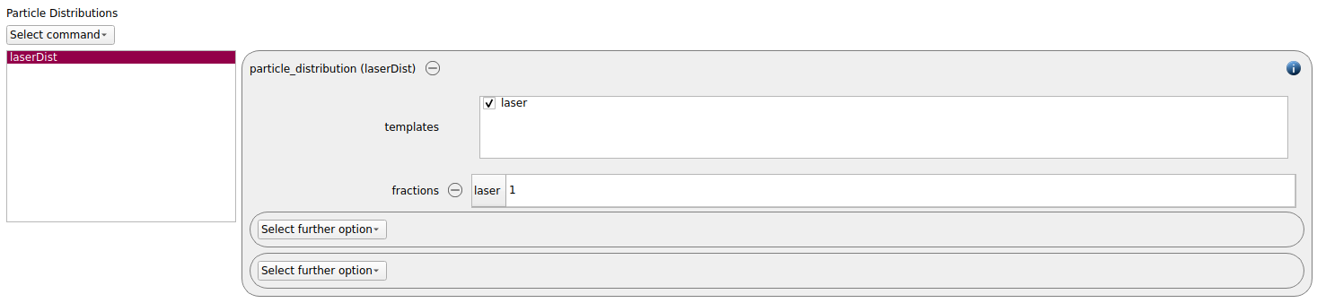
We also add the particle distributions:

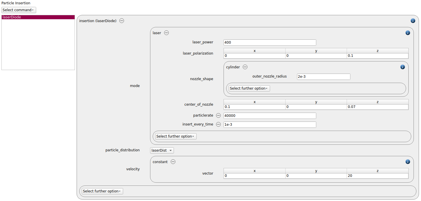
We use a laser insertion command, with the setting show in figure :

Simulation control

In this tab, we first define the time-step settings such as the desired simulation timestep of 1e-5 seconds and the total simulation time of 1 second. Per default also the check_timestep command command is enabled, which throws a warning when the time step exceeds 10 % of the Rayleigh or the Hertz time. These thresholds can be changed by setting an alternative value for hertz_fraction or rayleigh_fraction.

Running the simulation

After completing the setup and saving it, the simulation can be launched. Change to the Simulation view and set the number of cores to use to 2. First hit the “Check settings” button, and if the check returns “Check settings successfully completed” the simulation can be run by hitting “Run simulation”.

Postprocessing with Paraview

After the simulation is completed, all data written with the output_settings command can be visualized automatically by going to the Visualization view and hitting the “Start Paraview” button.

The image below shows the final state of the system: