Home
HomeEmptying of a container in a chamber with a 6dof lid
This tutorial consists of four simulations: first, a container is filled with particles. In the seconds simulation the container moves to another location. Then the container is tilted to allow for its emptying. In the last simulation the mesh motion is stopped and the motion of the particles as well as of the lid inside the container is calculated:
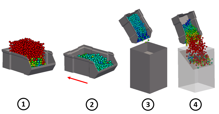
Name of the case: Project_6dof_container
Filling of the container
As a first step, the used materials command as well as the simulation domain are defined in the General Settings tab. Please note that in case of multiple dependent simulations, the dimensions of the simulation domain can only be defined in the first simulation. This means that the box forming the simulation domain has to be chosen big enough from the beginning.
General settings
In this simulation we set particles of particle shape sphere:

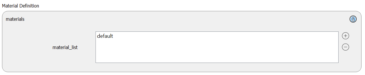
A single material with the name default is used:
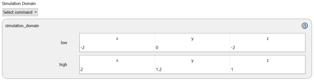
The simulation domain with x dimension ranging from -2 to 2 m, y dimension ranging from 0 to 1.2 m and z dimension ranging from -2 to 1 m:
Meshes and regions
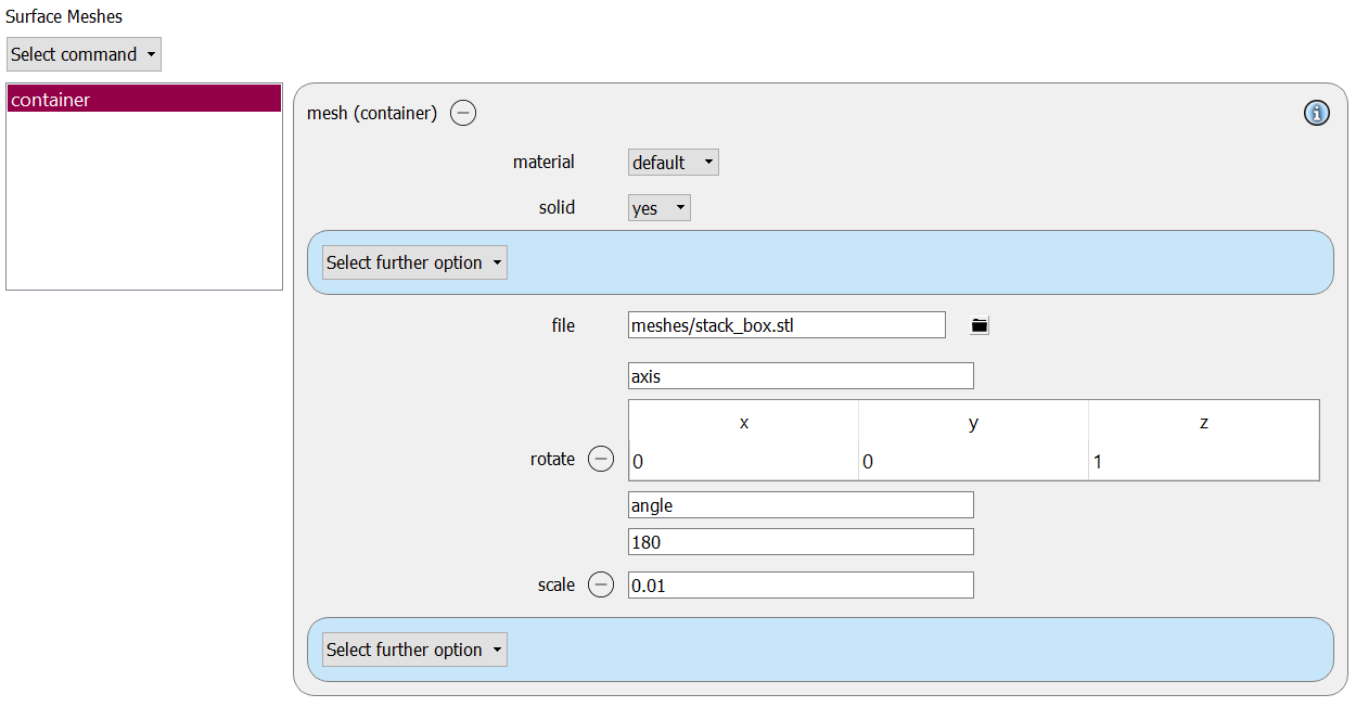
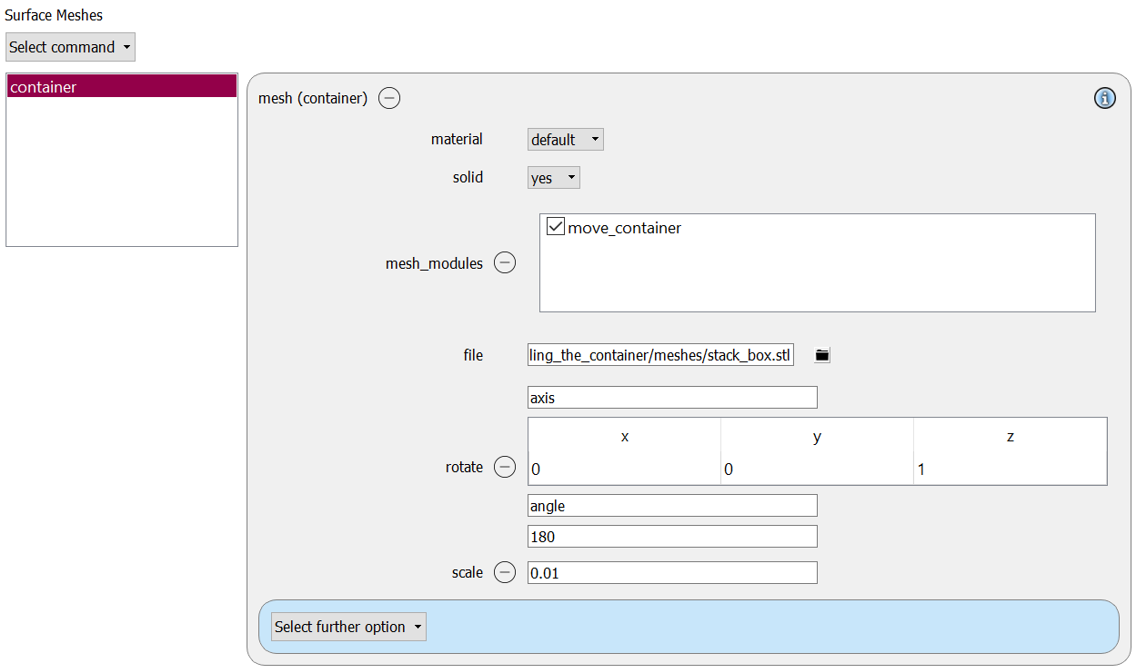
In the first simulation only the mesh command for the container is needed. The loaded mesh file is rotated 180 degrees around the z-axis and scaled by a factor of 0.01.
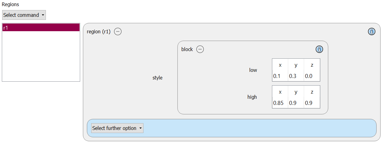
A block-shaped region command with dimensions 0.1 to 0.85 along x, 0.3 to 0.9 along y, and 0 to 0.9 along z is defined for particle insertion:
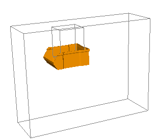
The container, the insertion region and the simulation domain can be seen in the 3D preview:
Physics models
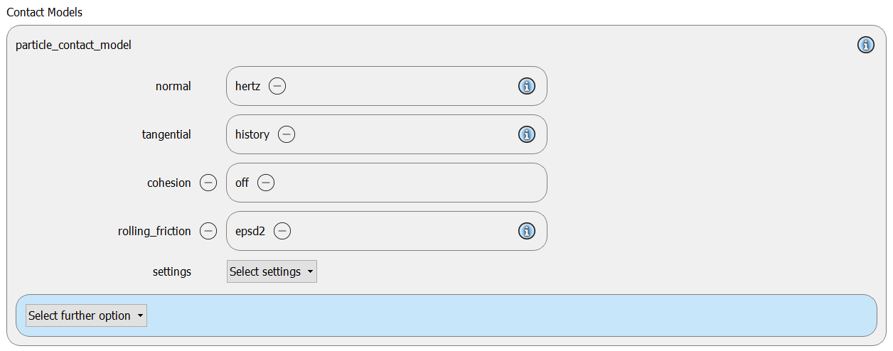
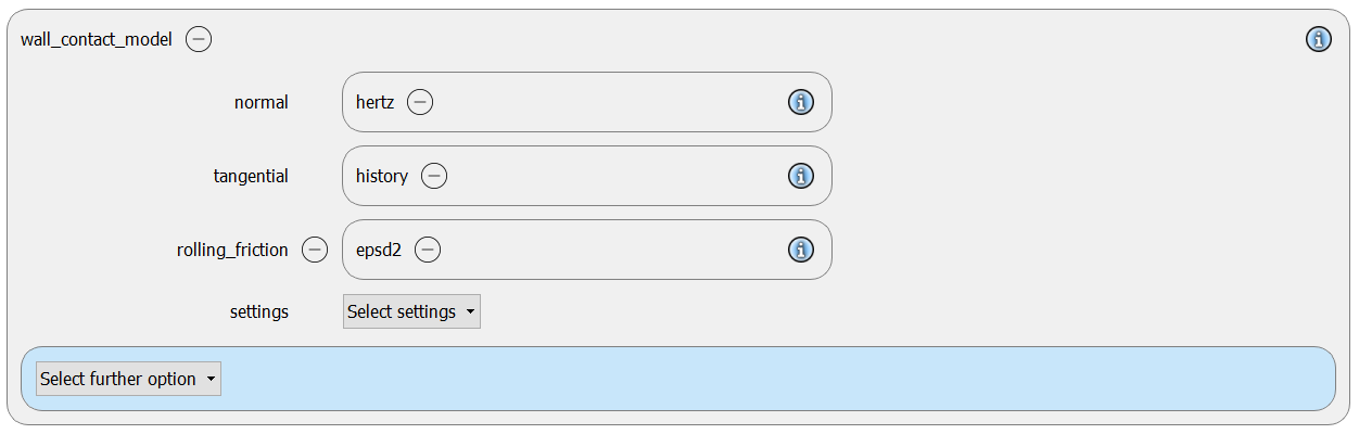
The contact models are now defined. For the particles we use the normal contact model hertz, the tangential model history and the rolling friction model epsd2:
Since we added a mesh in the previous section, a wall contact model is also added automatically to this section. We use the same properties as for the particle contact model:
Please note that for physical reasons the contact models cannot be changed in derived simulations.
Finally, gravity is enabled:

Per default gravity has a magnitude of 9.807 and acts into negative z-direction. These defaults can be changed by either setting the magnitude or the direction manually.
Particles
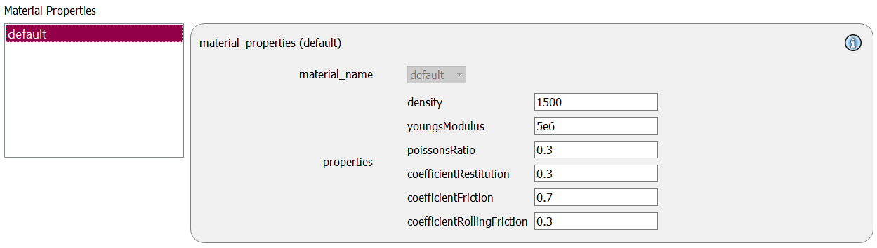
In the general settings tab we only defined a single material type (default), whose settings have to be specified here:
default |
|
Density |
1500 |
Young’s modulus |
5e6 |
Poisson’s ratio |
0.3 |
Coefficient of restitution |
0.3 |
Coefficient of friction |
0.7 |
Coefficient of rolling friction |
0.3 |
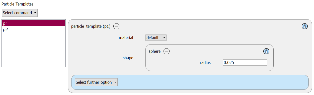
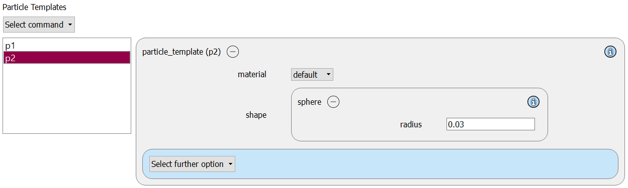
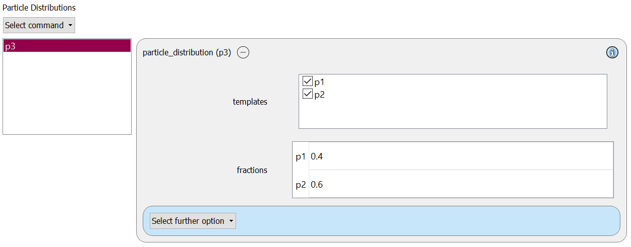
Two particle templates with radii of 0.025 and 0.03 m are generated and combined into a 40%-60% particle distribution:
A pack of particles with a velocity of 1 m/s in negative z-direction is inserted:
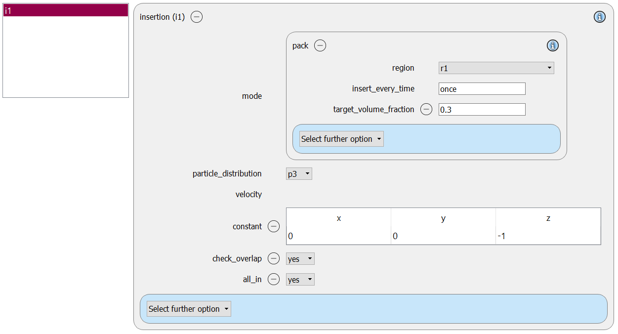
A volumefraction of 0.3 is selected, futhermore check_overlap and all_in are set to yes. The insert_every_time is set to once, i.e. the defined pack is only inserted once.
Simulation control
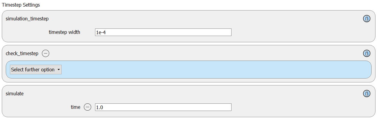
In this tab, we first define the time-step settings such as the desired simulation timestep of 1e-4 seconds and the total simulation time of 1 seconds. Per default also the check_timestep command command is enabled, which throws a warning when the time step exceeds 10 % of the Rayleigh or the Hertz time. These thresholds can be changed by setting an alternative value for hertz_fraction or rayleigh_fraction.
Output settings
In this tab, we first define the time-step width for the file and the terminal output:
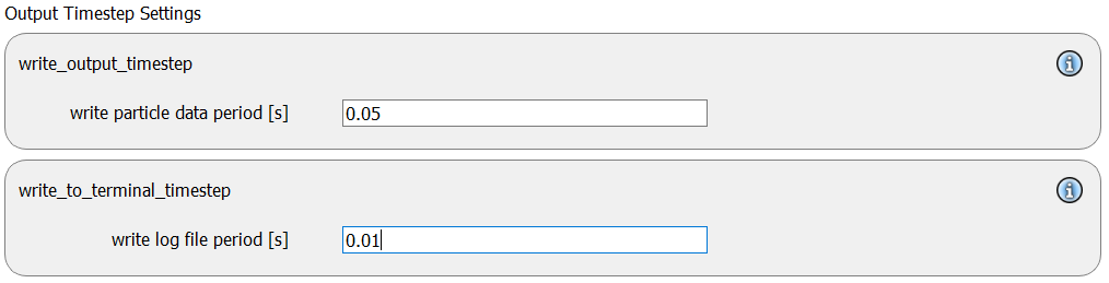
The output_settings command command takes care that all particle information and the meshes are written to files. Furthermore, it triggers the output of global quantities such as the kinetic energy of the particles or total normal and shear stresses onto meshes to the terminal. Please note that if the output of per-cell information on meshes such as wear, velocity of stress are desired, one has to add the keyword mesh_properties and select the required output.

Running the simulation
After completing the setup and saving it, the simulation can be launched. Hence, change to the Simulation view. First hit the “Check settings” button, and if the check returns “Check settings successfully completed” the simulation can be run by hitting “Start”:
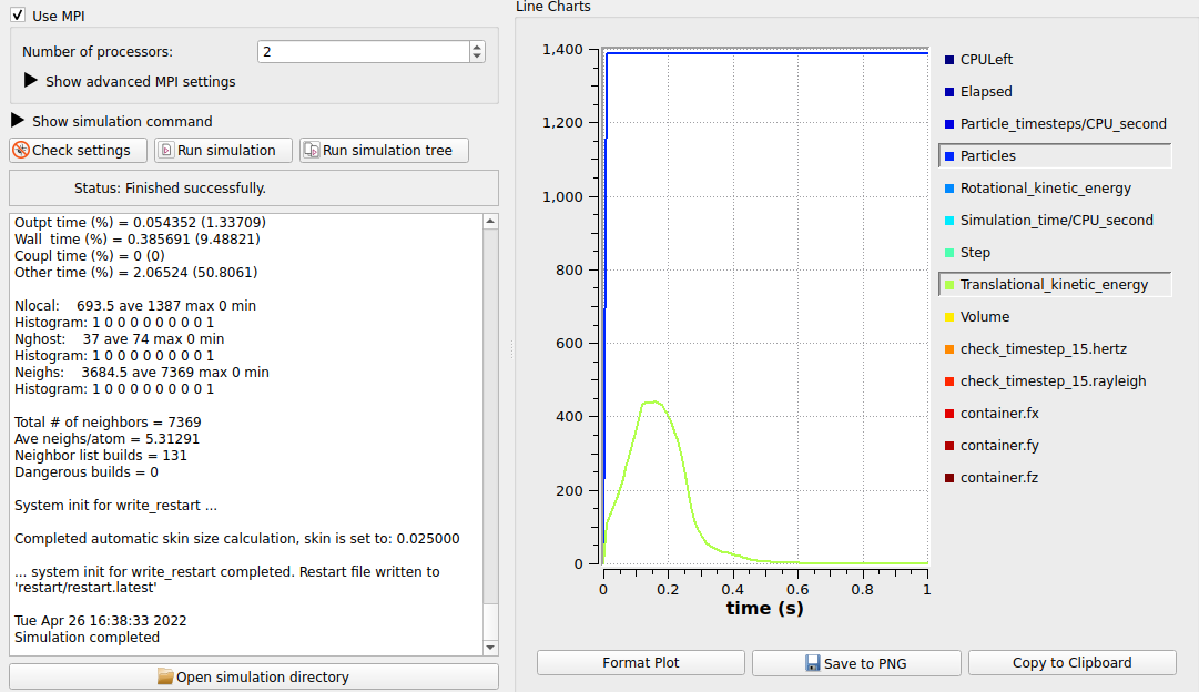
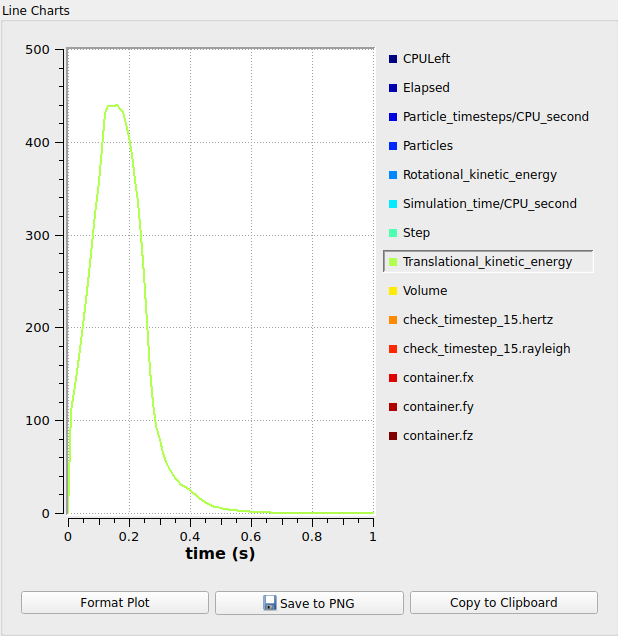
The graph shows that the number of particles remains constant throughout the simulation and if one considers the kinetic energy it shows that the settling process is completed after one second:
Postprocessing with Paraview
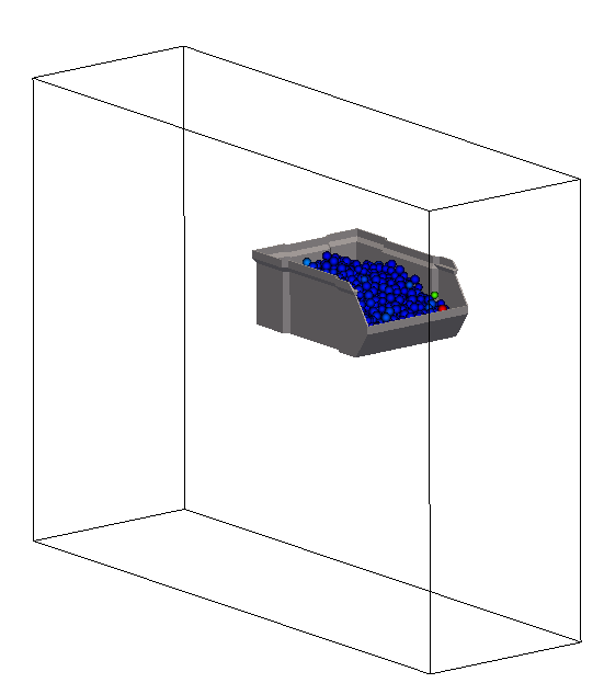
After the simulation is completed, all data written with the output_settings command can be visualized automatically by going to the Visualization view and hitting the “Start Paraview” button. The image below shows the final state of the case:
Moving the container
The filled container should now be moved with 1 m/s in negative x direction.
Removing the particle insertion command
To generate a simulation that is based on the results of the first one, the “Derive simulation” button underneath the simulation in the timeline has to be hit. This leads to a locking of the original simulation (i.e., nothing can be changed there anymore) and the generation of a new simulation. The particle shape, the name and number of materials, as well as the simulation domain size and the contact models cannot be modified in the derived simulation.
Since no further particles will be inserted, the insertion commands as well as particle distribution, particle templates and insertion region can be deleted. Please note that a command can only be deleted, if no other command depends on it. Therefore the mentioned order has to be kept when removing all insertion-related components.
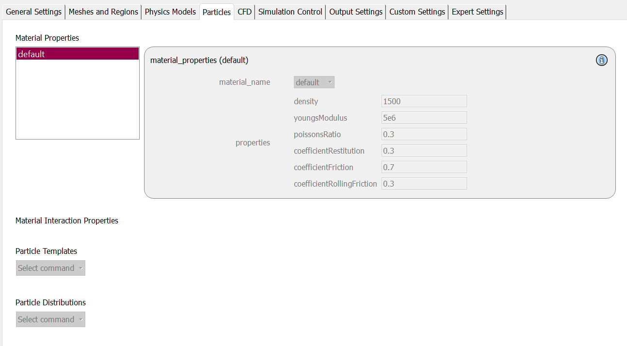
The particles tab below contains now only the particle properties:
Applying the mesh motion
In order to translate the container in the x-direction, a new mesh module must be added to the Meshes and Regions tab:
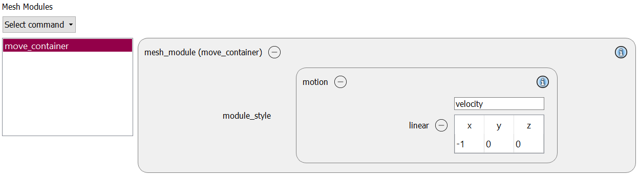
The newly generated mesh module has to be selected in the mesh_modules property of the container mesh:
If not already done, the insertion region can be removed in this tab.
Simulation control
The simulation time remains one second as in the previous case:
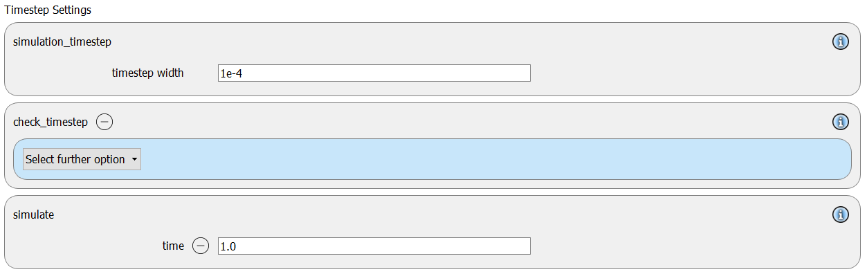
In the Scalability and Speed section of this tab we add the enable_loadbalancing command option:

Running the simulation
After completing the changes, the simulation can be launched in the simulation view:
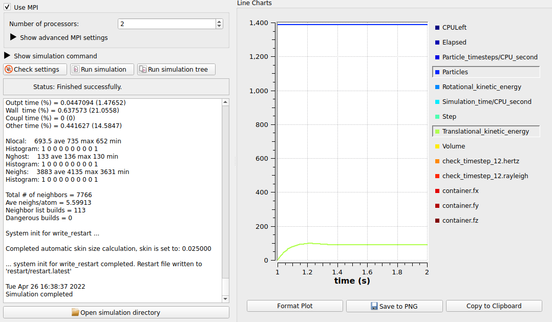
The number of particles remains constant, whereas the kinetic energy reaches a constant level after an initial increase.
Postprocessing with Paraview
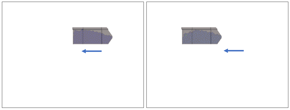
The motion of the container with the granular material can be visualized in Paraview (left: position of the container at the beginning of the simulation, right position at the last time step):
Tilting the container
As soon as the translational motion of the container is completed, another simulation is derived, in which the container will be tilted. In this simulation a new mesh modules and two additional meshes will be included and the existing translational mesh motion module will be changed to a rotational one.
Meshes and mesh motion
In the Meshes and Regions tab we start by adding a new 6-dof mesh module that will transform an inserted plate into a lid with a suspension force:
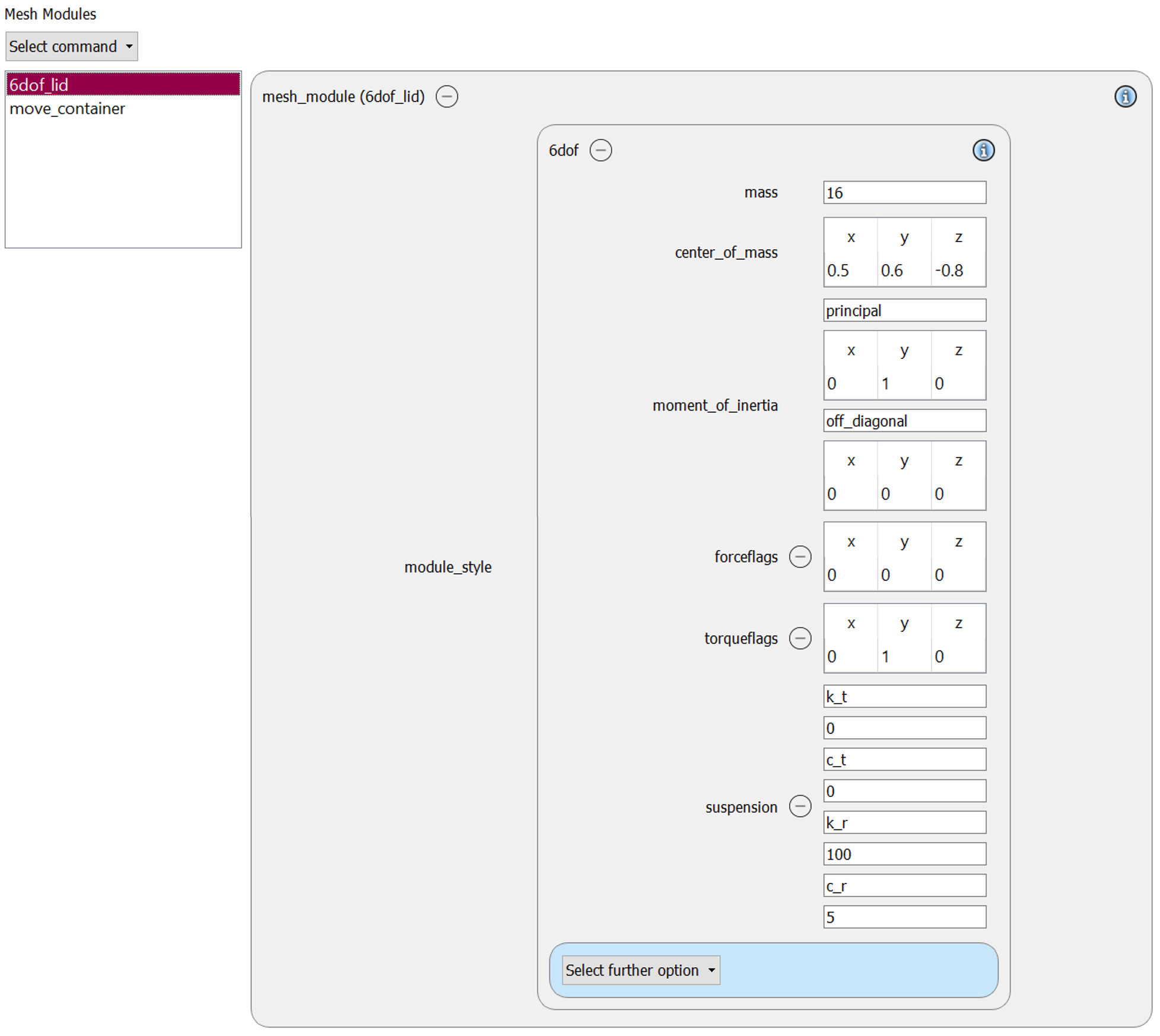
The center of mass of the plate (to be inserted later on) is set to (0.5, 0.6, -0.8), its mass is 16 kg, the Iyy value of the moment of inertia is 1, while all the other values are 0. Except the torqueflag around the y-axis, all other force- and torqueflags are zero, which disable any motion except a rotation around the y-axis. By selecting the keyword suspension, an additional suspension force and torque are added with a rotational stiffness of 100 and a rotational damping of 5.
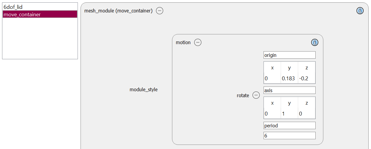
The mesh module motion is changed from a translational motion to a rotational one with a period of 6 seconds around the y-axis. The center of rotation is given by (0, 0.183, -0.2):
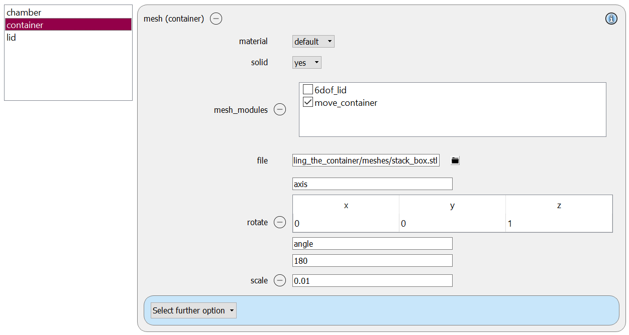
In the meshes section we leave the motion module activated:
Then we add a new mesh command, that forms a chamber, in which the particles will fall.
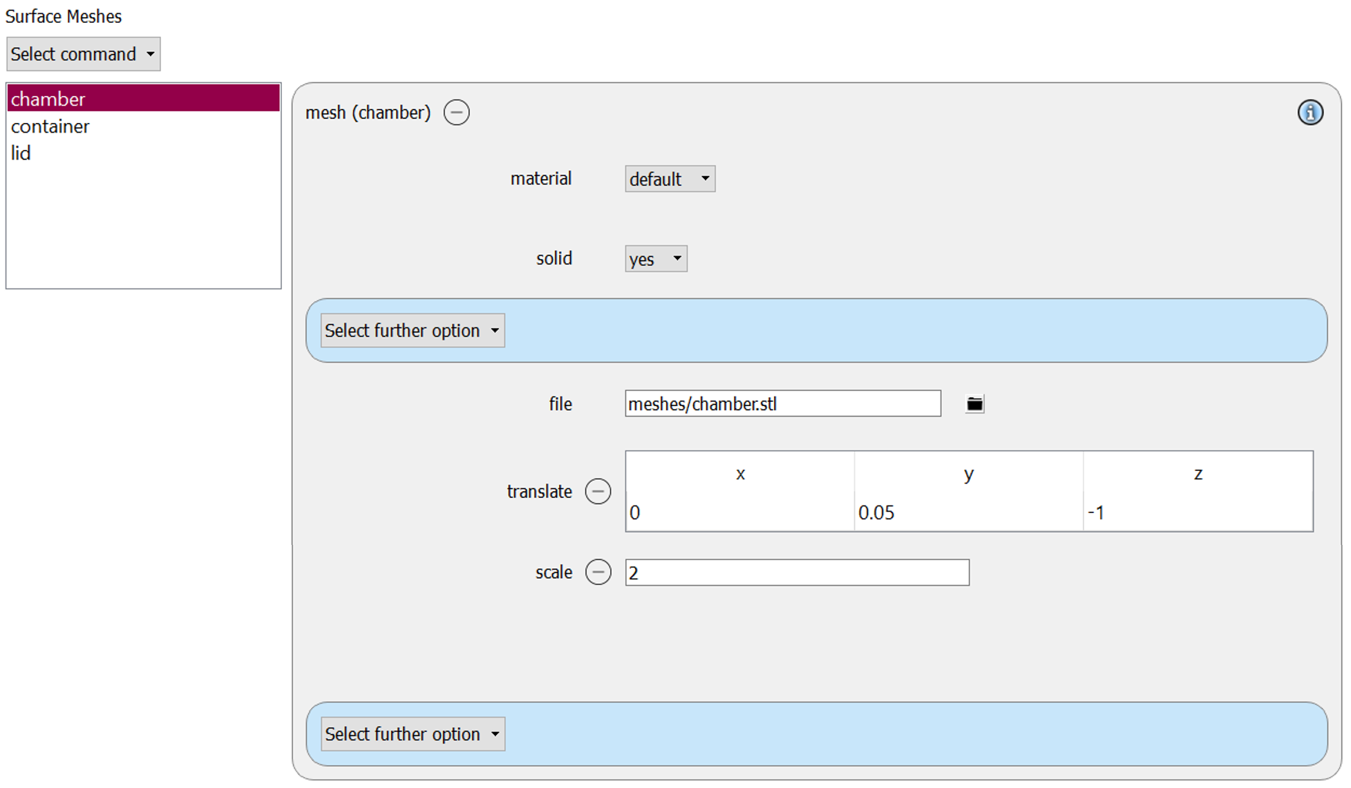
The chamber has to be moved by 0.05 m in y direction and -1 m in z direction and scaled by a factor of 2.
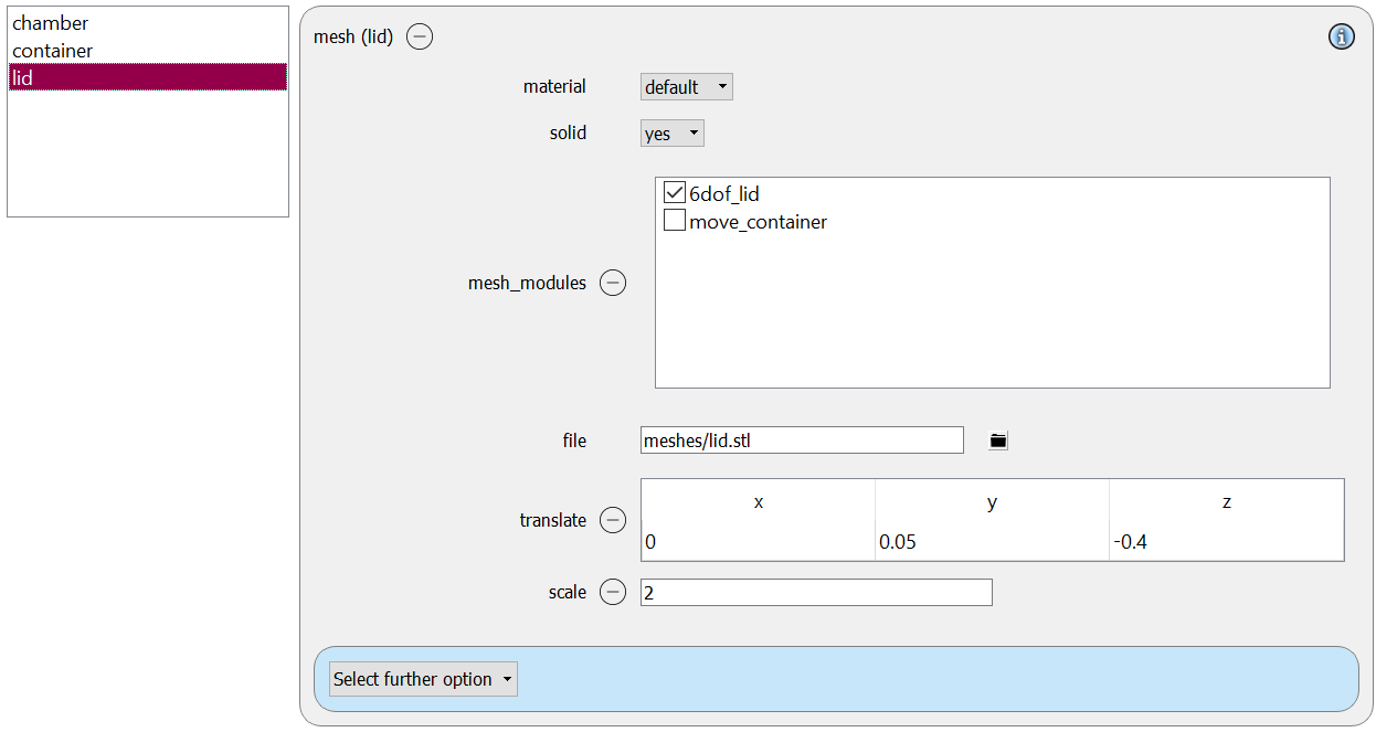
Then, the lid is finally inserted, which has to be translated by 0.05 m in y and -0.4 m in z-direction and scaled by a factor of 2. Furthermore, the 6dof mesh module has to be selected:
Simulation
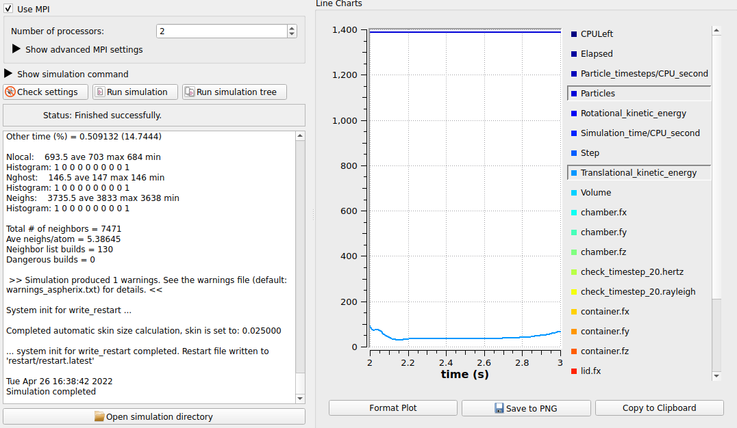
The simulation can be launched now. While the number of particles remains constant, the kinetic energy increases:
Postprocessing with Paraview
The results can be visualized in Paraview:
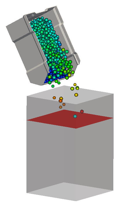
Since the motion of the particles due to the tilting of the container has just started, another simulation is derived:
Emptying the container
In this simulation the motion of the container is stopped, and the interaction of the particles with the 6dof lid is considered.
Stopping the container motion
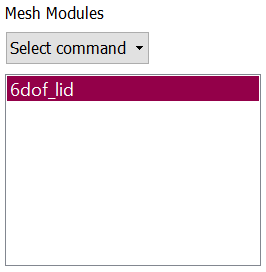
In the Meshes and Regions tab the mesh module for the motion is removed:
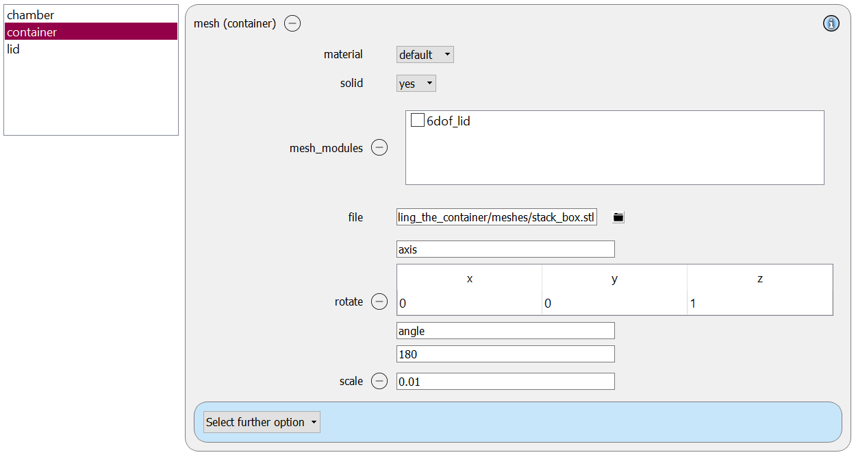
The container mesh is now left without mesh module:
Increasing the runtime
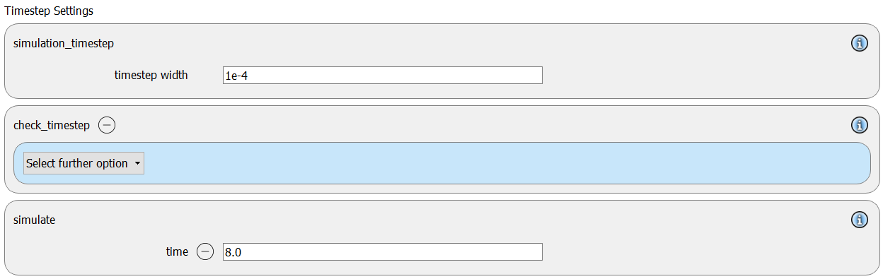
In the Simulation Control tab we increase the runtime from 1 second to 8 seconds:
Simulation
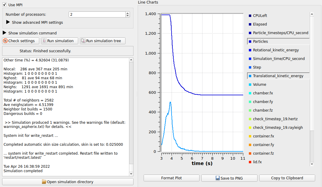
After these two small changes the simulation can be launched. The plots show that the number of particles increases first and reaches a constant level, at which the kinetic energy becomes zero:
Postprocessing with Paraview
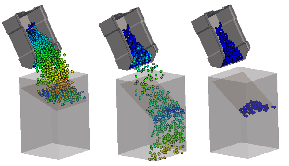
The results can again be visualized in Paraview, the below image shows the system at three different points in time: