Evaluating the external work on a geometry

This tutorial consists of two simulations. In the first one a dense packing of spheres is created using the “simulate until settled” command. In the second case a bucket digs into the particle packing, and the external work (total, force, torque) on the component is evaluated.

In this tutorial a cube is inserted at the same time as a pack of particles and they both settle under the influence of gravity.

Name of the case: Project_External_work

Simulation 1 - Creating a packing of spheres

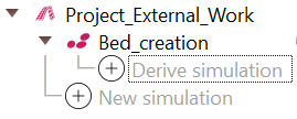
We start with generating a new project and adding a simulation to it:

As a first step, the used materials command as well as the simulation domain are defined in the General Settings tab. Please note that in case of multiple dependent simulations, the dimensions of the simulation domain can only be defined in the first simulation. This means that the box forming the simulation domain has to be chosen big enough from the beginning.

General settings

In this simulation we set particles of particle shape sphere:

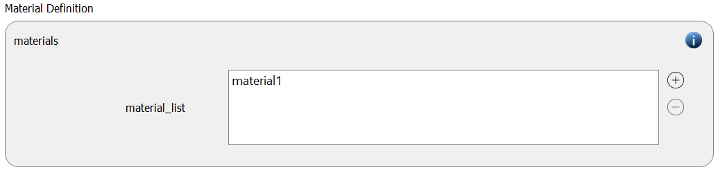
In this simulation only one material type is used (here called default):

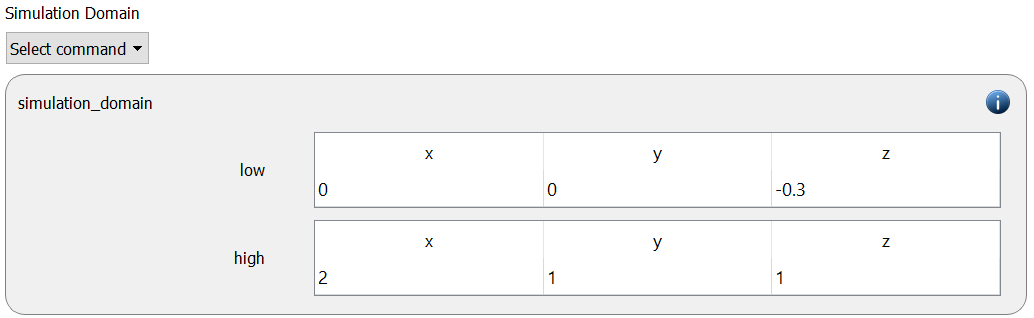
The simulation domain with x dimensions ranging from 0 to 2, y dimensions ranging from 0 to 1 and z dimentions ranging from -0.3 to 1 is created:

Meshes and regions

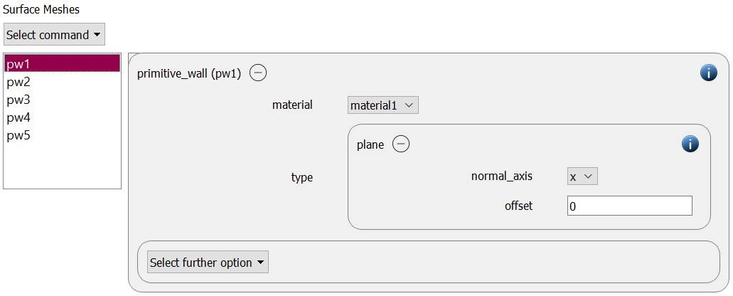
Five primitive walls of type plane are used to keep the particles inside the simulation domain (x: 0 and 2, y: 0 and 1, z: 0):

Physics models

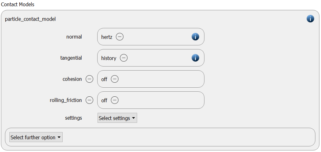
The contact models are now defined. For the particles we use the normal contact model hertz and the tangential model history.

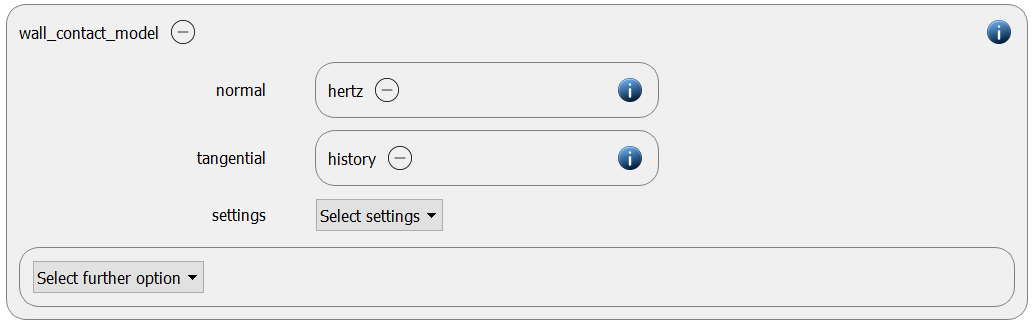
Since we added primitive walls in the previous section, a wall contact model is also added automatically to this section. We use the normal contact hertz and the tangential model history:

Finally, the gravity is enabled:

Per default the gravity has a magnitude of 9.807 and acts into negative z-direction. These defaults can be changed by either setting the magnitude or the direction manually.

Particles

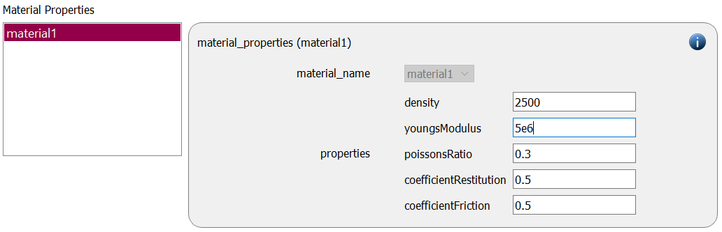
In the general settings tab we only defined a single material type (default), whose settings have to be specified here:

	default
Density	2500
Young’s modulus	5e6
Poisson’s ratio	0.3
Coefficient of restitution	0.5
Coefficient of friction	0.5

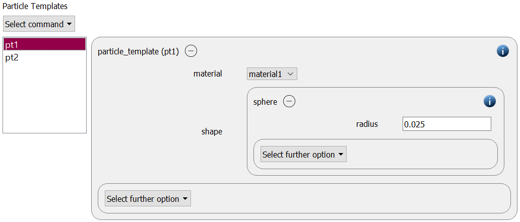
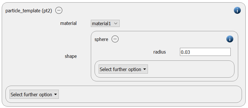
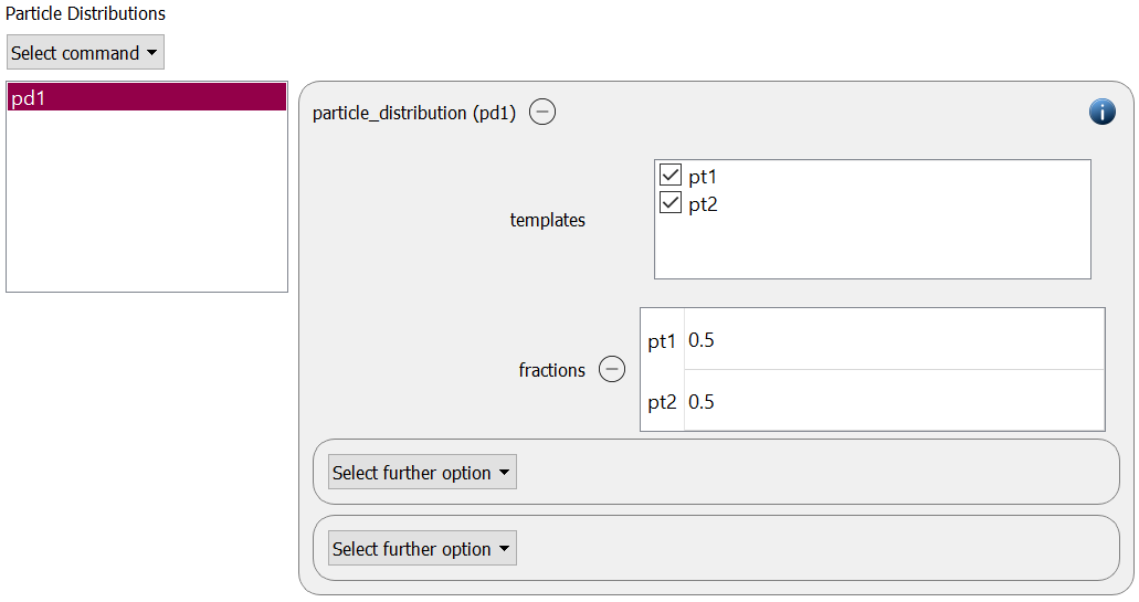
Two particle templates with a radius of 0.025 and 0.03 m are generated and used to form a particle distribution:

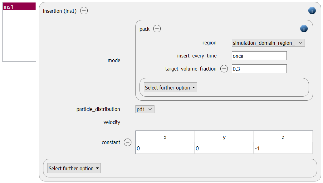
A pack of particles with a velocity of 1 m/s in negative z-direction is inserted using an insertion command command with mode pack:

Simulation control

In this tab, we first define the time-step settings such as the desired simulation timestep of 1e-4 seconds. Instead of defining a total run time we use the simulate command command in mode “until:settled”. In this mode the simulation runs until the kinetic energy in the simulation domain (or a defined region) falls below a certain threshold. The user can, but does not have to, define the threshold. Per default also the check_timestep command command is enabled, which throws a warning when the time step exceeds 10 % of the Rayleigh or the Hertz time. These thresholds can be changed by setting an alternative value for hertz_fraction or rayleigh_fraction.

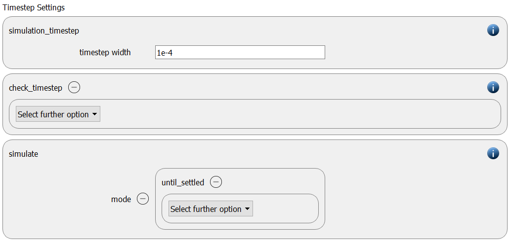
If no doc:neighbor lists <solver:neighbor_list> skin size is defined, Aspherix sets this value automatically. For optimizing the parallelization behaviour for non-parallel runs, the enable_loadbalancing command command is used:

Output settings

In this tab we first define the timestep width for the file and the terminal output:

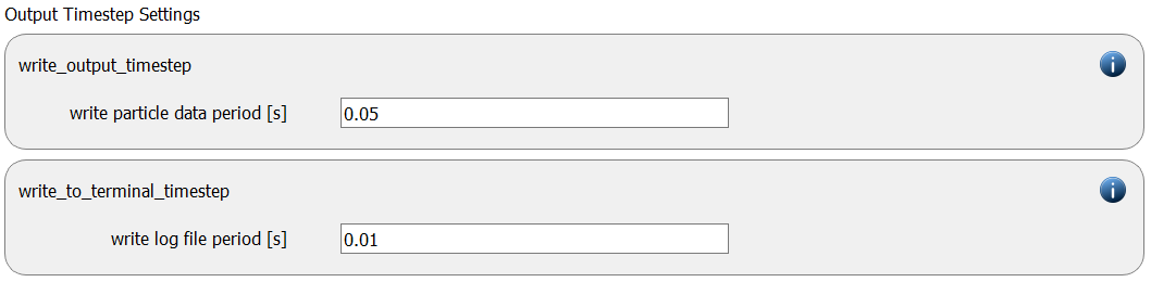
The output_settings command command the takes care that all particle information and the meshes are written to files accordingly. Furthermore it triggers the output of global quantities such as the kinetic energy of the particles or total normal and shear stresses onto meshes to the terminal. Please note that if the output of per-cell information on meshes such as wear, velocity of stress are desired, one has to add the keyword mesh_properties and select the required output.

Running the simulation

After completing the setup and saving it, the simulation can be launched. Hence, change to the Simulation view. First hit the “Check settings” button, and if the check returns “Check settings successfully completed” the simulation can be run by hitting “Start”:

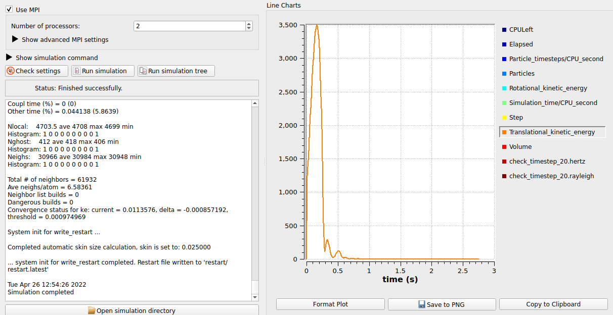
The graph shows that the simulation runs for a bit over 2.5 seconds until the kinetic energy falls below the internally defined threshold.

Simulation 2 - Digging

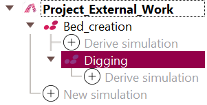
We carry on with deriving a simulation from the base case:

Meshes and regions

In this simulation we include a bucket that follows a predefined motion path (translational and rotational displacements). We start with defining a mesh_module for the mesh motion:

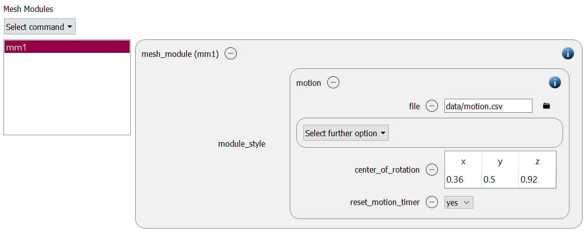
The motion file looks as following (details about the required format can be found in the documentation):

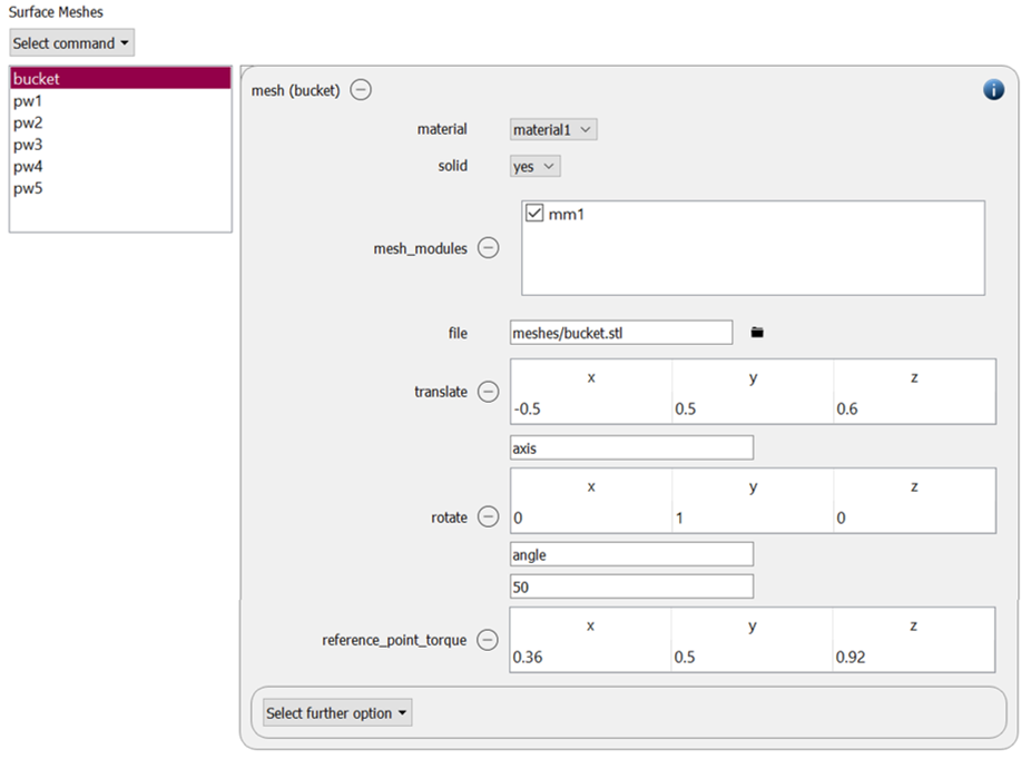
In the next step the geometry for the bucket is loaded and conntected with the mesh motion:

Particles

The particle insertion command can be removed:

This step is a case-cleanup step, since the insertion command is completed it has not further effect.

Simulation control

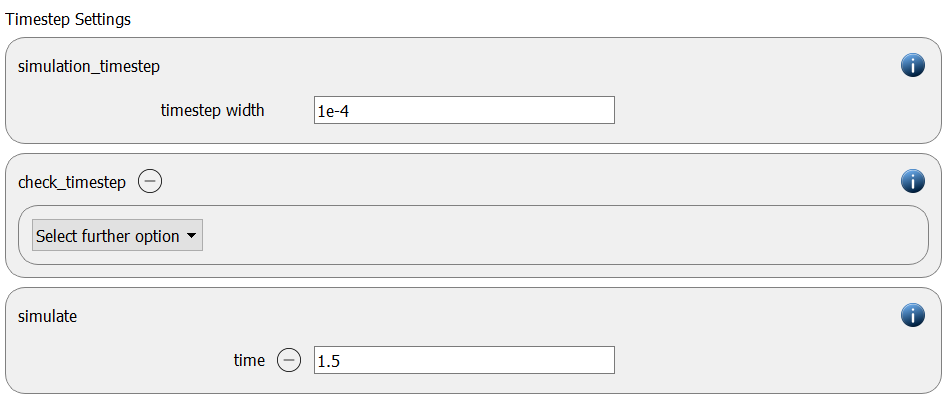
The simulation time is changed to 1.5 seconds:

Output settings

In this section we add three commands for evaluating the external work that acts onto the bucket. The first command (id: cal1) calculates the total work, the second command (id: cal2) shows the component of the work that is caused by torque and the third command (id: cal3) shows the force-induced part of the work:

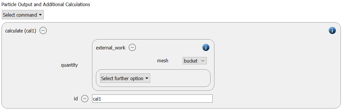
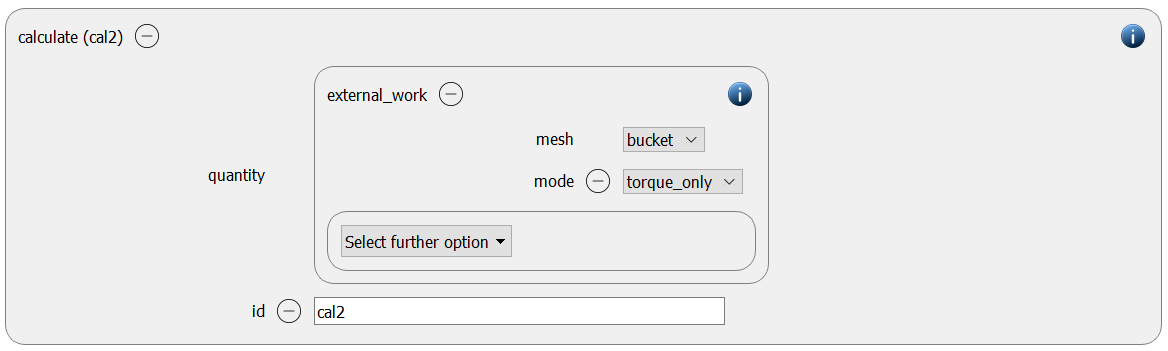
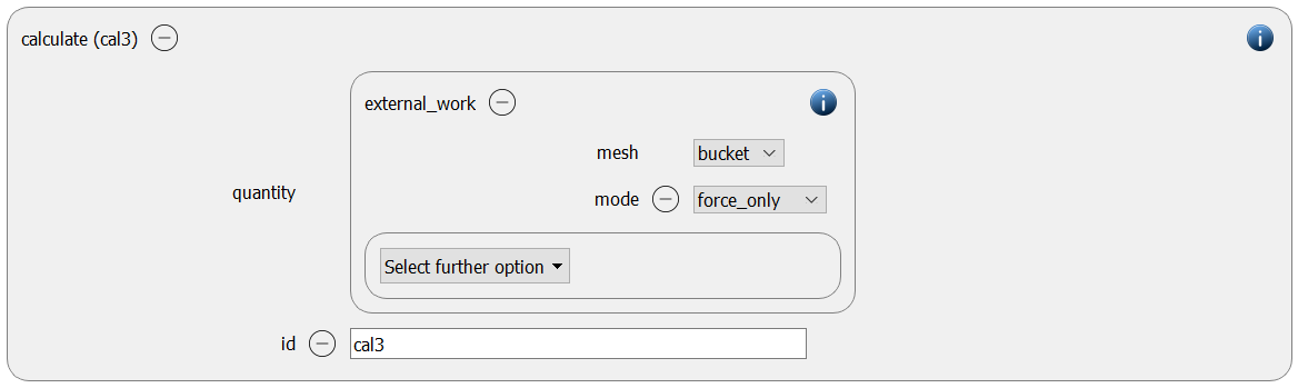
Please make sure that the keyword id is added. With this handle it is possible to use a write_to_file command command in the expert settings for saving the output of this calculation to a text file (weight 23), furthermore the output of the command can be visulized in the graph during the simulation (see below).

Running the simulation

After completing the setup and saving it, the simulation can be launched. Hence, change to the Simulation view. First hit the “Check settings” button, and if the check returns “Check settings successfully completed” the simulation can be run by hitting “Start”:

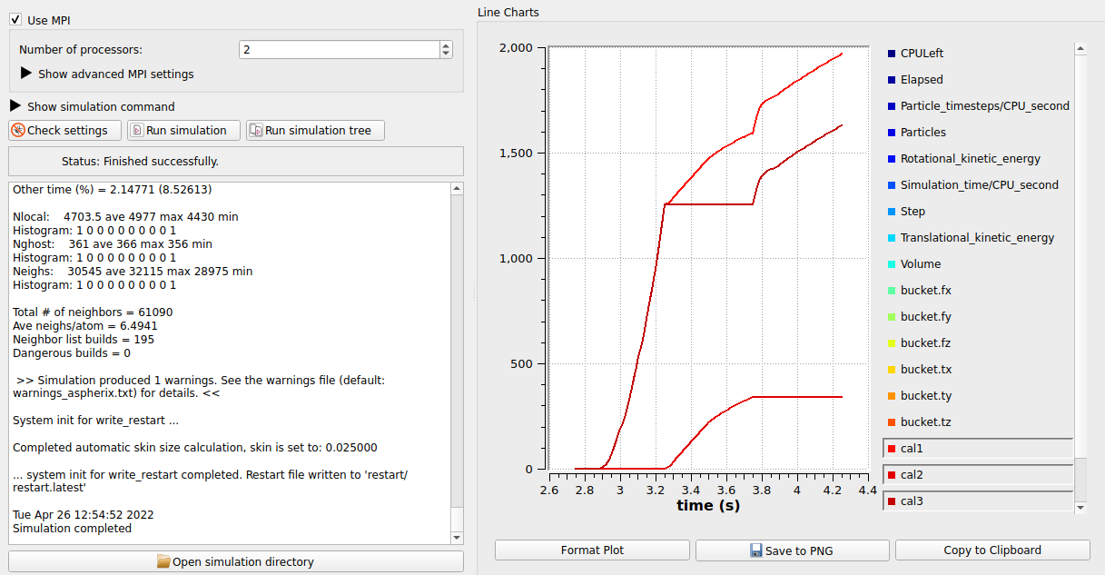
The graph shows the total external work as well as the work induced by force and torque only.

Postprocessing with Paraview

After the simulation is completed, all data written with the output_settings command can be visualized automatically by going to the Visualization view and hitting the “Start Paraview” button.

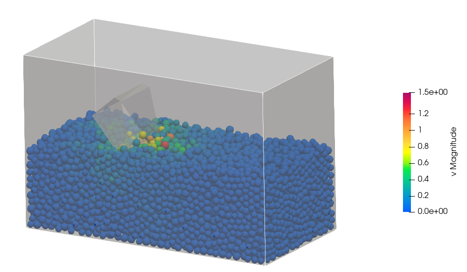
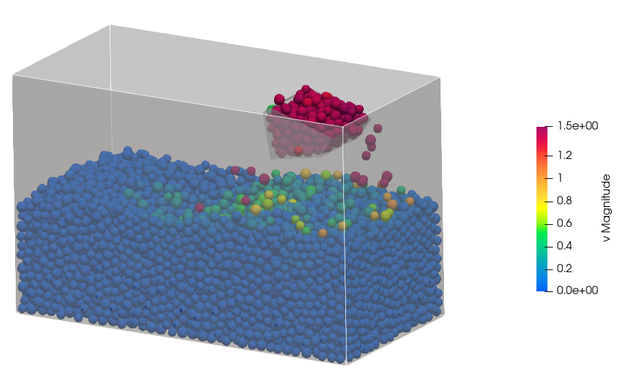
The images below show the state of the system at two different times - first shortly after the bucket made contact with the particle bed and second after some material has been excavated:

Name of the case: Project_External_work