6dof-cube falling into a particle bed

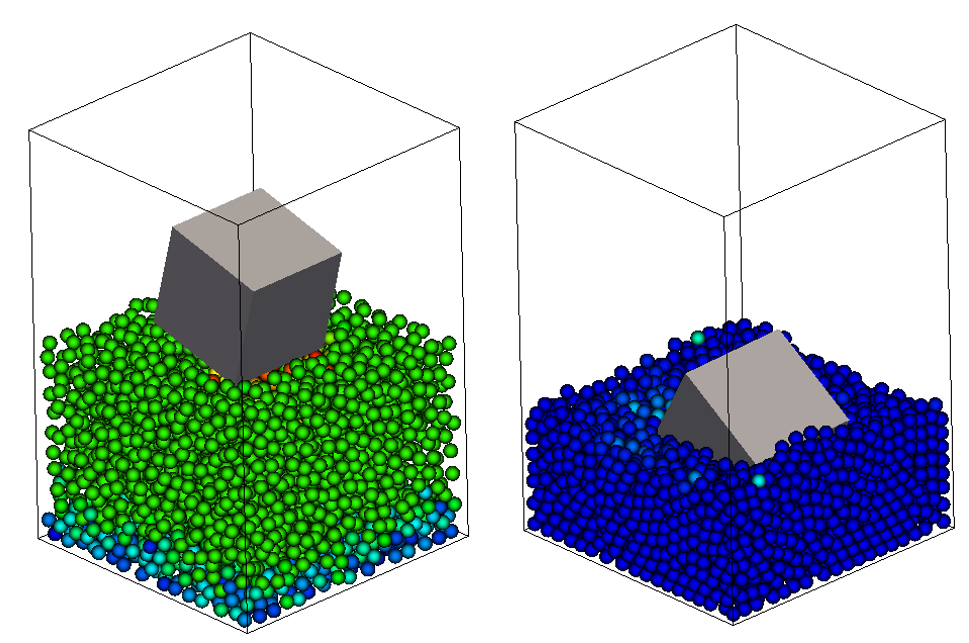
In this tutorial a cube is inserted at the same time as a pack of particles and they both settle under the influence of gravity.

Name of the case: Project_6dof_cube

Setting up the Aspherix(R) GUI simulation

As a first step, the used materials command as well as the simulation domain are defined in the General Settings tab. Please note that in case of multiple dependent simulations, the dimensions of the simulation domain can only be defined in the first simulation. This means that the box forming the simulation domain has to be chosen big enough from the beginning.

General settings

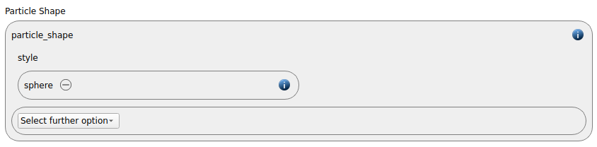
In this simulation we set particles of particle shape sphere:

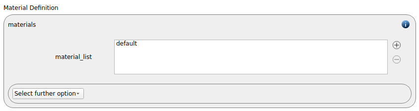
In this simulation only one material type is used (here called default):

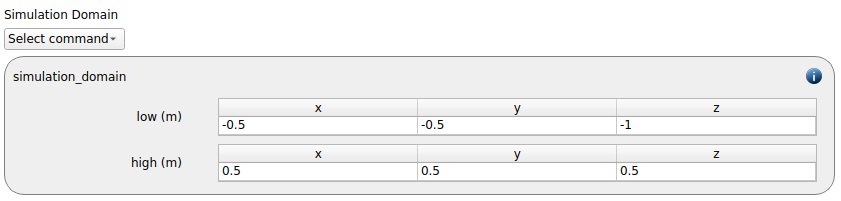
The simulation domain with x and y dimensions ranging from -0.5 to 0.5 and z dimension ranging from -1 to 0.5 is created:

Meshes and regions

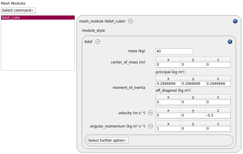
We start creating a 6dof mesh module for the settling cube. The center of mass is defined as (0, 0, 0), while the mass of the object is 40 kg. The principal moments of inertia are (0.266666, 0.266666, 0.266666), while the off-diagonal moments of inertia are all zero. The initial falling velocity is equal to -0.5 m/2 in z-direction and the angular momentum around the x-axis is 1 kg m^2 s^-1:

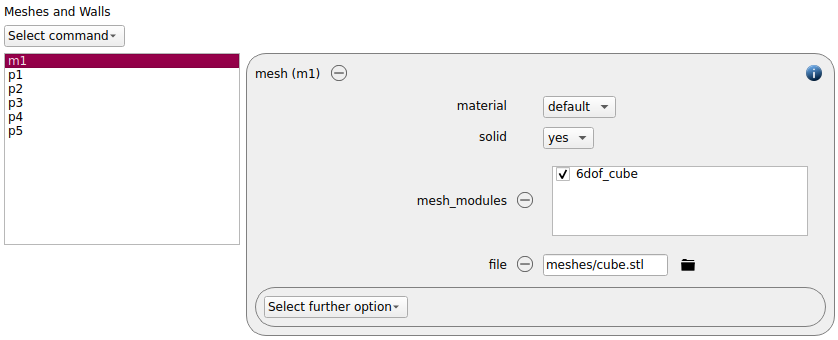
Next, we load the geometry of the cube via the mesh command command:

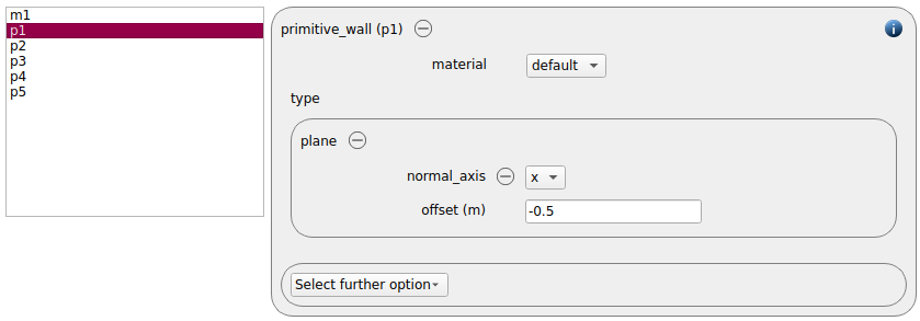
Then, five primitive walls are created to keep the inserted particles from leaving the simulation domain:

plane name	normal axis	offset
p1	x	-0.5
p2	x	0.5
p3	y	-0.5
p4	y	0.5
p5	z	-1.0

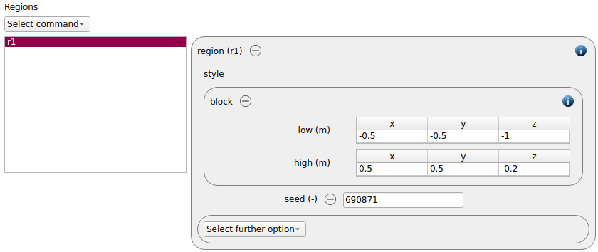
A block-shaped region command with the dimensions -0.5 to 0.5 in x and y dimension and -1 to 0.2 in z dimension is defined for the particle insertion

Both the cube and the region can be seen in the 3D preview:

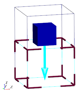
The preview in this case also already shows the insertion.

Physics models

The contact models are now defined. For the particles we use the normal contact model hooke and the tangential model history.

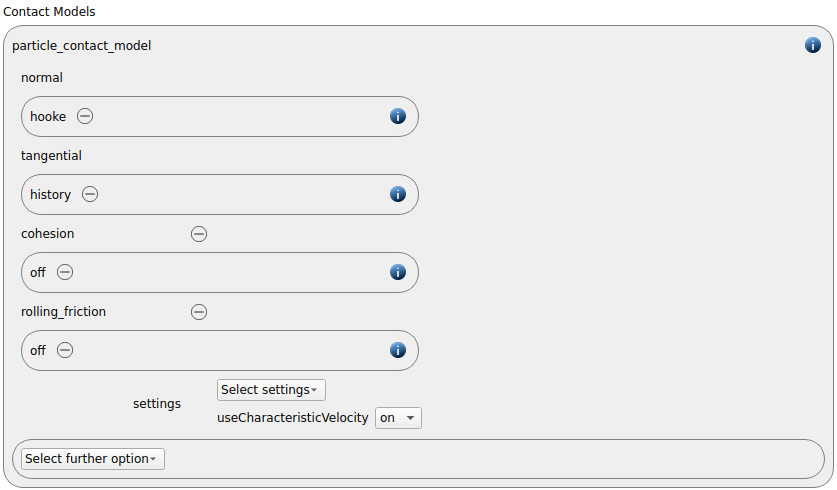
Since we added a mesh and primitive walls in the previous section, a wall contact model is also added automatically to this section. We use the same contact models as for the particle-particle interactions:

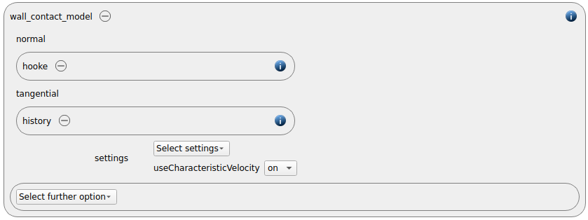
In both cases the hooke model is used with the setting useCharacteristicVelocity on.

Finally, the gravity is enabled:

Per default the gravity has a magnitude of 9.807 and acts into negative z-direction. These defaults can be changed by either setting the magnitude or the direction manually.

Particles

In the general settings tab we only defined a single material type (default), whose settings have to be specified here:

	default
Density	1000
Young’s modulus	5e6
Poisson’s ratio	0.45
Coefficient of restitution	0.7
Coefficient of friction	0.05

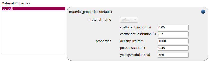
The characteristic velocity entry is required when the hooke model is selected:

A particle template with a radius of 0.025 m is generated and used to form a particle distribution:

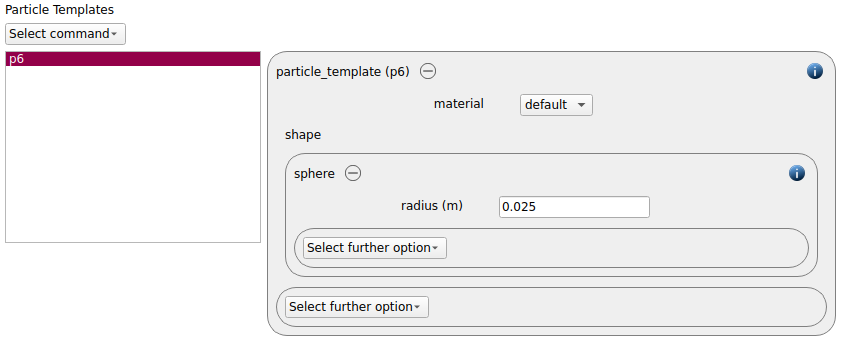
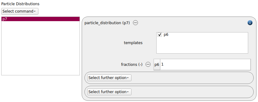
A pack of particles with a velocity of 0.2 m/s in negative z-direction is inserted using an insertion command command with mode pack:

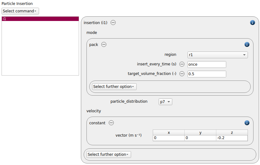
The selected target voidfraction of 0.5 is relatively high, it is thus possible that the inserted amount of particles is lower than the requested amount. For particle distributions that consist of a single template this has no effect; however, if the distribution consists of several templates, the proportion between the particle types might not be maintained. The insert_every_time is set to once, ensuring that the pack is inserted only once at the beginning.

Simulation control

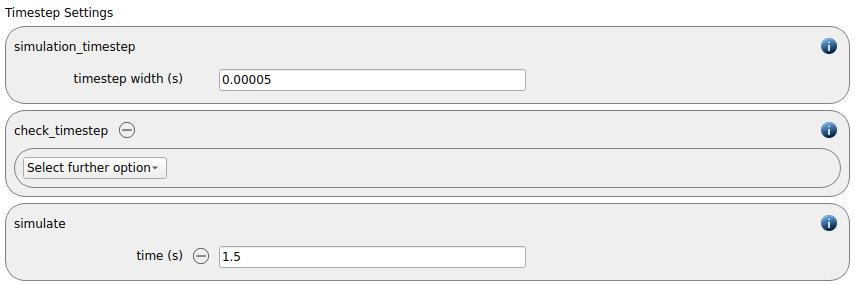
In this tab, we first define the time-step settings such as the desired simulation timestep of 5e-5 seconds and the total simulation time of 1.5 seconds. Per default also the check_timestep command command is enabled, which throws a warning when the time step exceeds 10 % of the Rayleigh or the Hertz time. These thresholds can be changed by setting an alternative value for hertz_fraction or rayleigh_fraction.

Output settings

In this tab we first define the timestep width for the file and the terminal output:

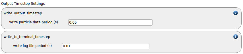
The output_settings command command the takes care that all particle information and the meshes are written to files accordingly. Furthermore it triggers the output of global quantities such as the kinetic energy of the particles or total normal and shear stresses onto meshes to the terminal. Please note that if the output of per-cell information on meshes such as wear, velocity of stress are desired, one has to add the keyword mesh_properties and select the required output.

Running the simulation

After completing the setup and saving it, the simulation can be launched. Hence, change to the Simulation view. First hit the “Check settings” button, and if the check returns “Check settings successfully completed” the simulation can be run by hitting “Start”:

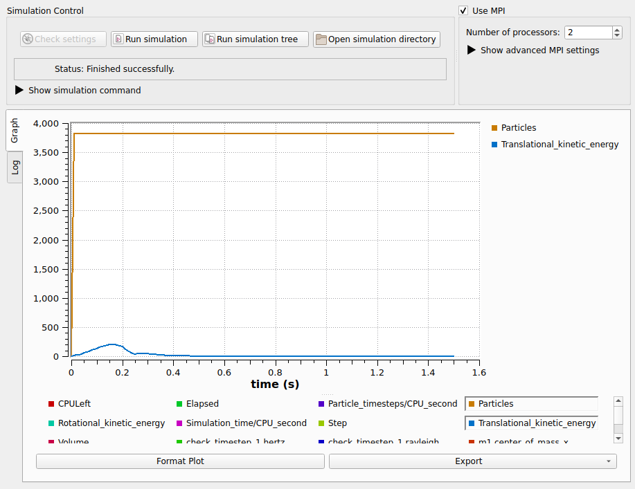
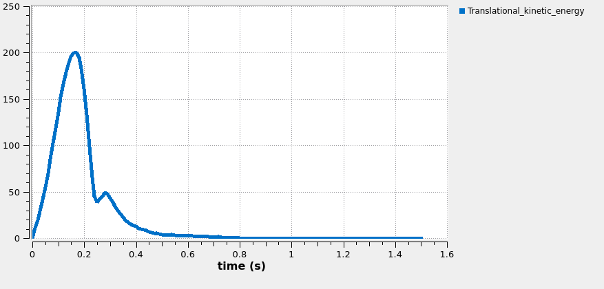
The graph shows that the insertion of the particles is completed after 30000 time steps (1.5 seconds), and if one considers the kinetic energy it shows that the settling process is completed after 1.5 seconds:

Postprocessing with Paraview

After the simulation is completed, all data written with the output_settings command can be visualized automatically by going to the Visualization view and hitting the “Start Paraview” button.

The images below show the state of the system at two different times - first short after the insertion of the settling and once when the process is completed: