Stream insertion of nonspherical particles until a region is filled

In this case we demonstrate the usage of the insertion stream_regionfill command in combination with facetted concave particles. The insertion command is active until a user-defined region contains a specified number of particles. The case is set up using the CGS unit system.

Name of the case: Project_Fill_Region

Simulation Setup

In this simulation concave facetted particles are inserted through a stream. The insertion will stop once the particle count in a specified region reaches a certain value. For easier post-processing the particles in the target region are marked and counted additionally.

General settings

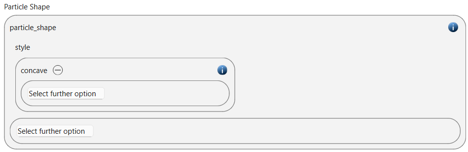
In this simulation we use particles of particle_shape command concave:

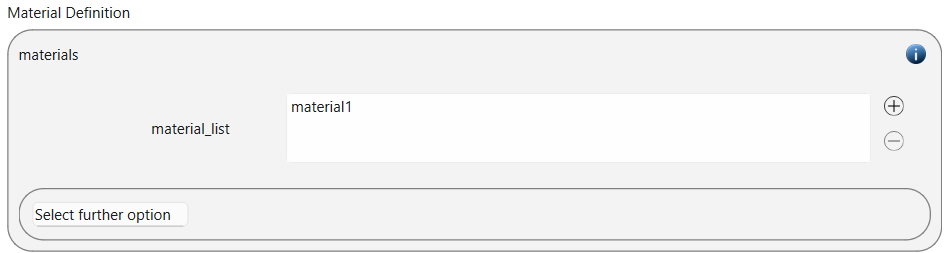
A material with name material1 is defined:

The units command are set to CGS:

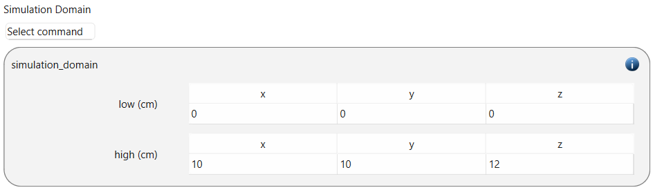
The simulation domain is defined with x and y-dimensions ranging from 0 to 10 cm and z-dimensions ranging from 0 to 12 cm:

Meshes and regions

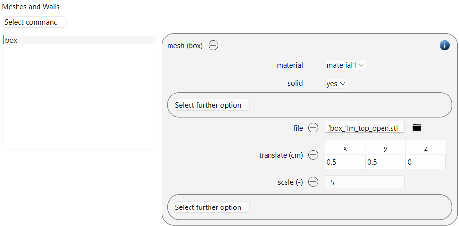
A box-shaped mesh command is inserted that is used as wall for capturing the particles in the target region:

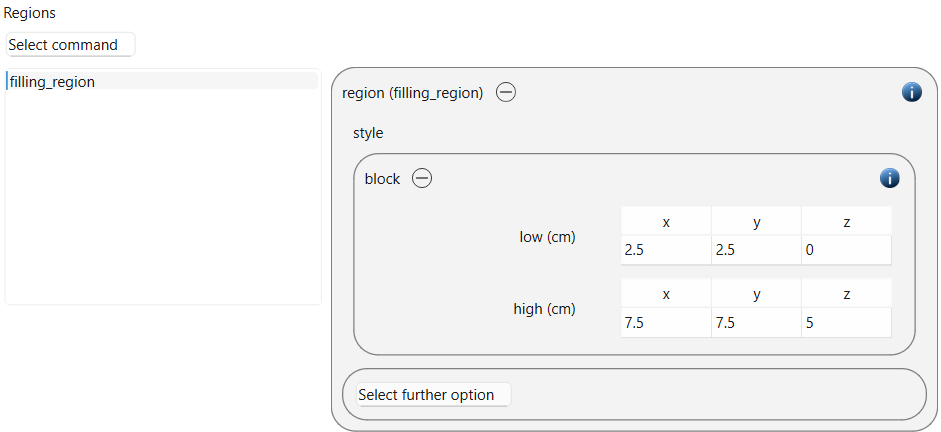
The target region command is defined as block, ranging from 2.2 to 7.5 cm in x and y-direction and from 0 to 5 cm in z-direction:

Physics models

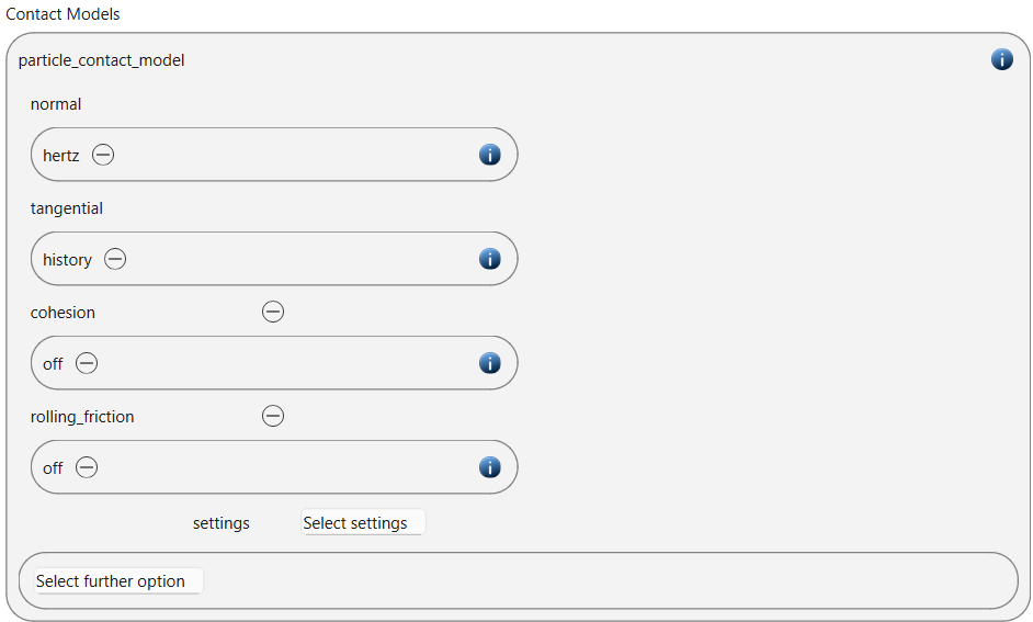
In the next step, the definition of the physics models takes place. For the particles we use the normal contact model hertz and the tangential model history.

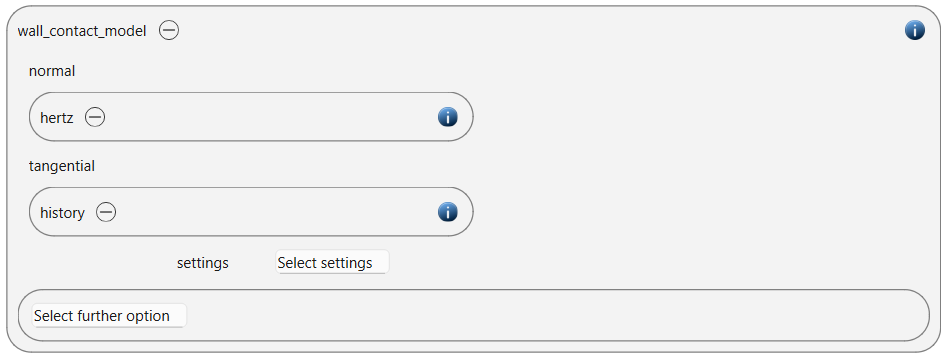
Since we added meshes in the previous section, also a wall contact model was added automatically in this section. We use the same contact models as for the particles:

Also the gravity is defined in this section:

Per default the gravity has a magnitude of 9.807 and acts into negative z-direction. These defaults can be changed by either setting the magnitude or the direction manually.

Particles

In the general settings tab we introduced two materials. Here we define the required material properties.

	material1
Density	1
Young’s modulus	5e7
Poisson ratio	0.3
Coefficient of restitution	0.5
Coefficient of friction	0.5

We are going to use concave facetted particles. Aspherix requires a specific input format (a clump of strictly convex particles) which can be generated with the concave builder (Tools / Nonspherical particles / Concave Builder), using an stl file as input:

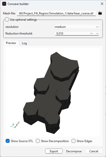
After a successful decomposition the generated data can be exported directly to the simulation. By pressing the “Export” button not only the data is stored in the correct place, but also the corresponding particle template is generated:

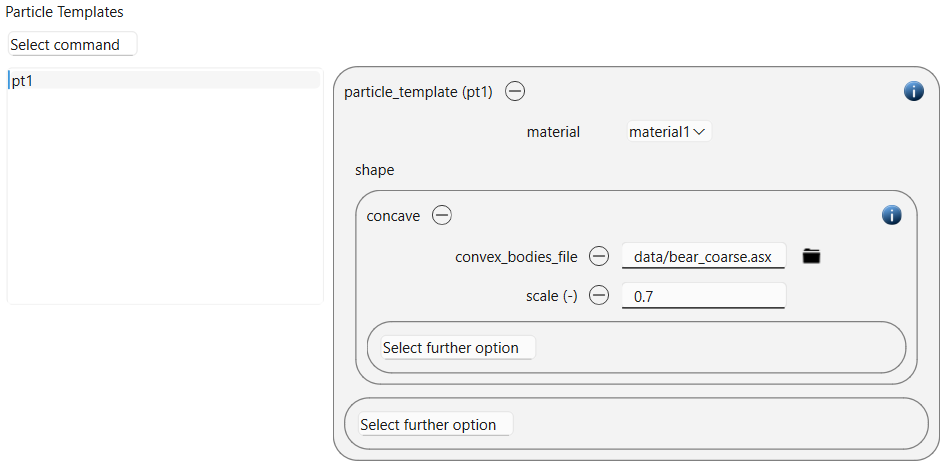
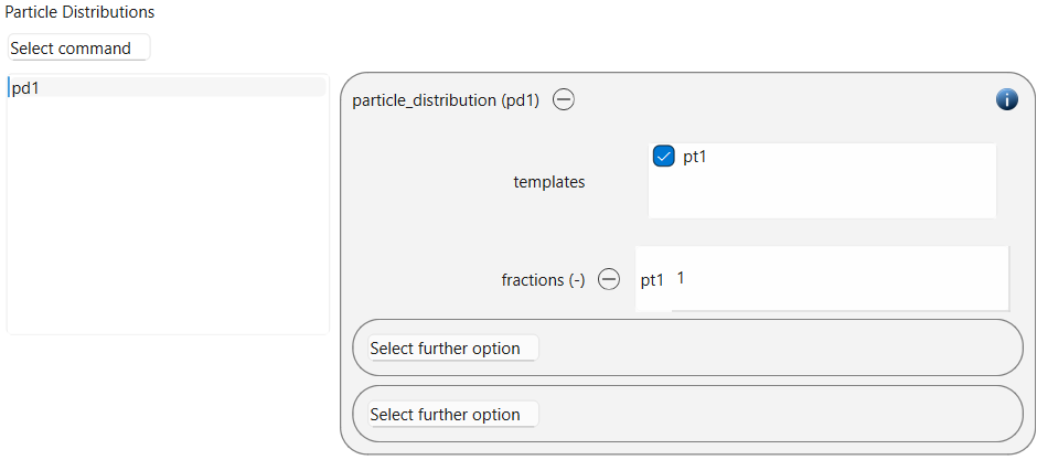
Please remove the previously already existing, empty particle template. This template is used to define a particle distribution:

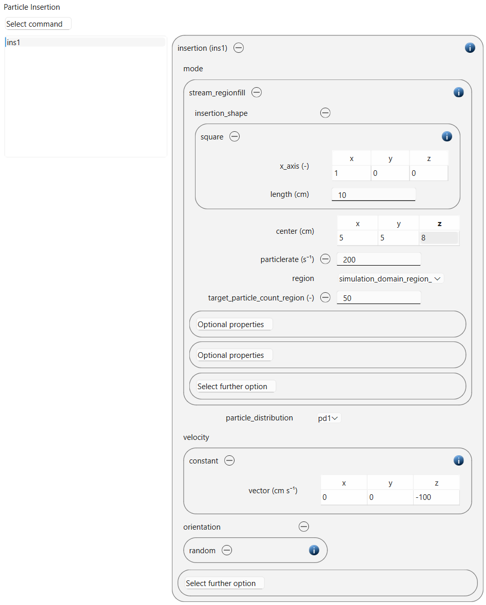
An insertion command command in mode stream_regionfill is used for particle insertion. For the stream insertion we use a square-shaped insertion shape, with a side length of 10 cm, an x-axis of (1,0,0) and a center of (5,5,8). The particle rate is 200 particles per second. The region to be observed is the filling_region that was defined before. The target particle count in the region is set to 50. The initial particle velocity is set to 100 cm/s in negative z-direction.

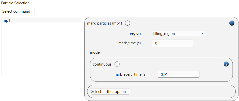
For being able to visually track the number of particles in the filling region we add a mark_particles command command:

Simulation control

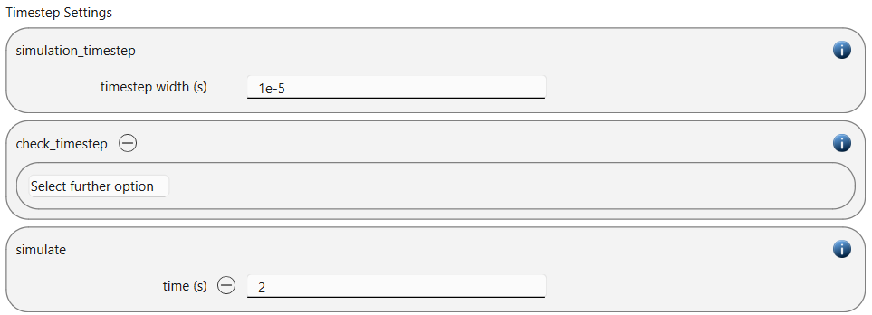
In this tab one first chooses the time step settings such as the desired simulation timestep of 1.e-5 seconds. With the simulate command command the total simulation time is set to 2 seconds. Per default also the check_timestep command command is enabled, which throws a warning when the time step exceeds 10 % of the Rayleigh or the Hertz timestep.

Output settings

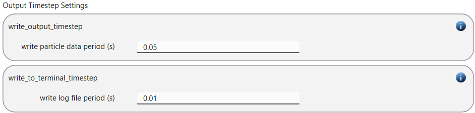
In this tab we first define the timestep width for the file and the terminal output:

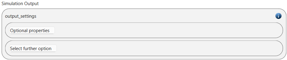
The output_settings command command takes care that all particle information and the meshes are written to files accordingly. Furthermore it triggers the output of global quantities such as the kinetic energy of the particles or total normal and shear stresses onto meshes in the terminal.

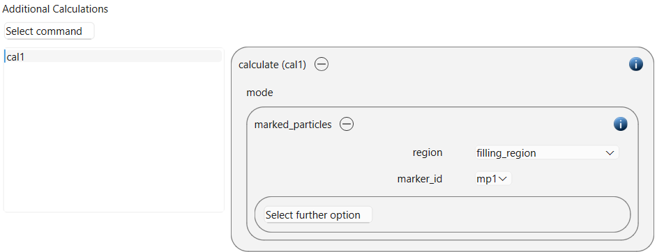
For getting the number of marked particles as global output we add a calculate marked_particles command:

Running the filling simulation

After saving the case we can change to the Simulation section. By hitting the Start button we can start running the simulation either serially or in parallel, using mpi. The loop script provides data for the number of particles, the kinetic energy, the total mass in the region and the kinetic energy in the region.

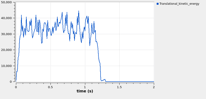
This graph shows the kinetic energy of all particles during the simulation:

This graph shows the total number of particles in the simulation as well as the number of marked particles (in the filling_region):

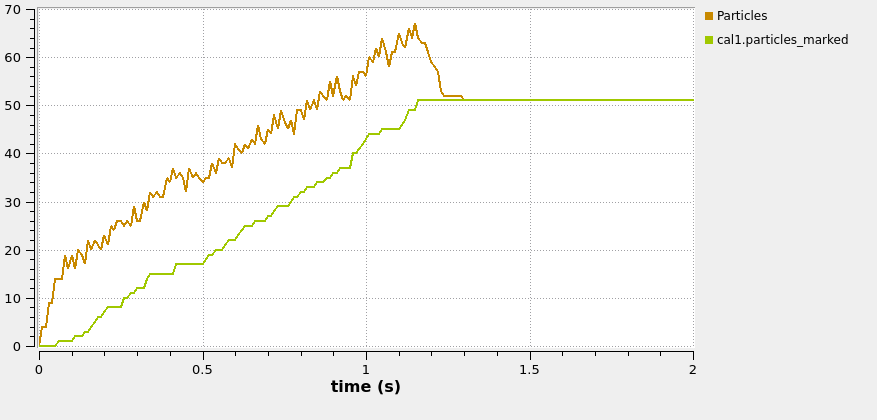
Since marked particles will not leave the filling_region again, the total number of marked particles and the number of marked particles coincide.

Result

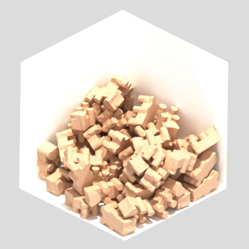
The result of the calculation can then be visualized with Paraview or Ovito. The image shows the state of the particle bed at the end of the simulation:

Name of the case: Project_Fill_Region