Rotating distributor: one-way coupling against MRF fluid field

In this tutorial particles are inserted above a rotating distributor. Two one-way coupling commands are applied, one in the proximity of the rotating distributor and another one in the far field. The command close to the rotating geometry consists of two zones. The inner zone is a cylinder, in which the provided velocity field is rotated with the given velocity (multi reference frame, MRF), whereas in the surrounding zone the velocities as given by the data file are applied. The one-way coupling command in the far field acts on a coarser grid and also uses a stationary velocity field.

The image shows the case setup:

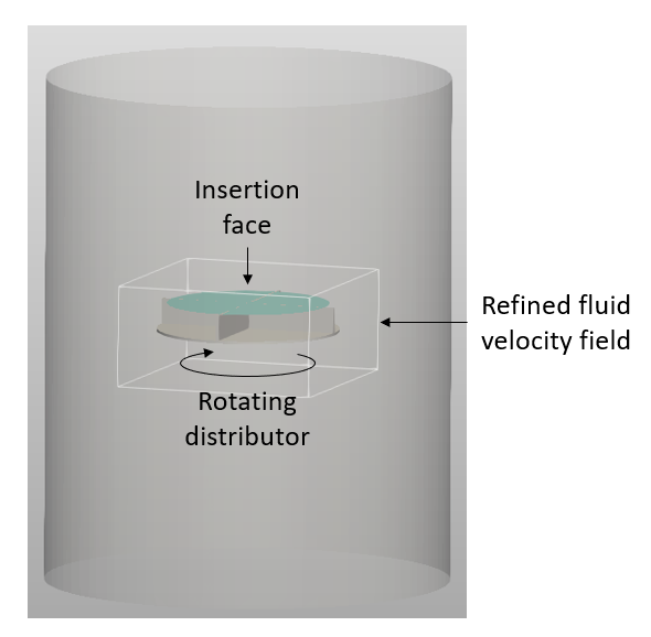
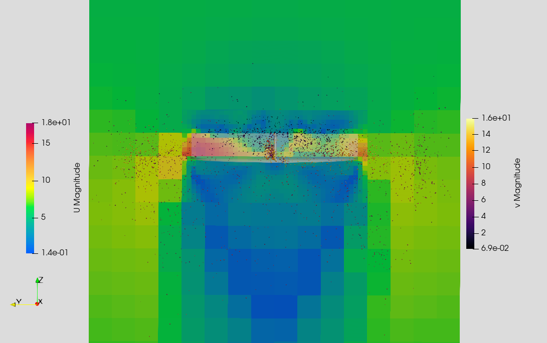
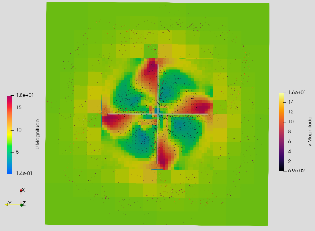
Particles are inserted at an insertion face directly above the rotating distributor. The fluid field in the proximity of the rotating distributor is refined, the remaining flow field is much coarser. A cylinder forms the outer boundary of the device. The image below shows the final state of the simulation. Please note that for the refined fluid velocity field a moving reference frame (MRF) is used, whereas the coarse velocity field remains constant. The particles are scaled up by a factor of three for better visibility.

Name of the case: Project_One_Way_Coupling_MRF

Setting up the simulation

As a first step, the particle shape, the used material and the simulation domain are defined in the General Settings tab. Please note that in case of multiple dependent simulations, the dimensions of the simulation domain can only be defined in the first simulation. This means that the box forming the simulation domain has to be chosen big enough from the beginning.

General settings

In this simulation we set particles of particle shape sphere:

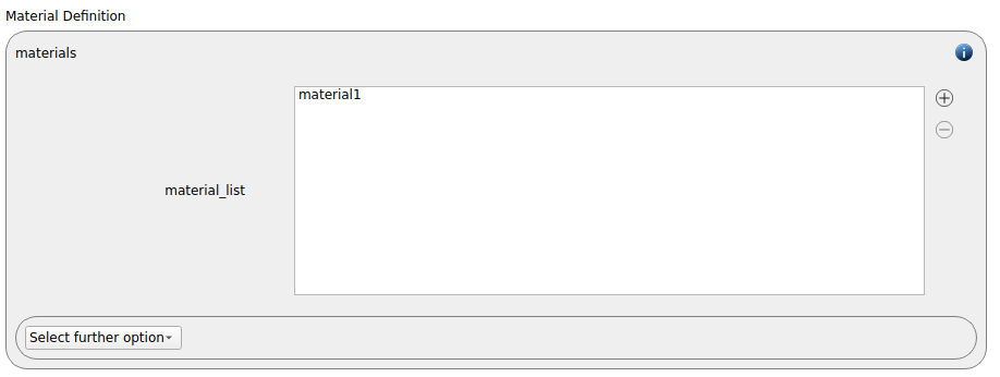
A single materials command with the name material1 is used:

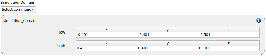
The simulation domain with x and y dimensions ranging from -0.401 to 0.401 and z dimensions ranging from -0.501 to 0.501 is created:

Meshes and regions

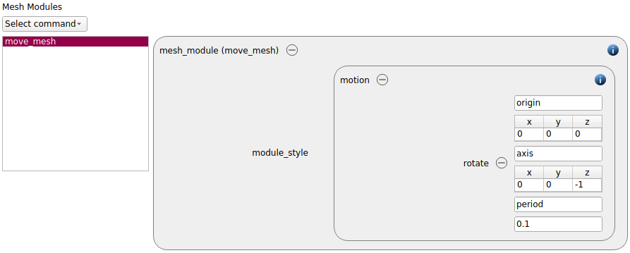
We start with defining the rotational motion of the distributor by adding a mesh_module

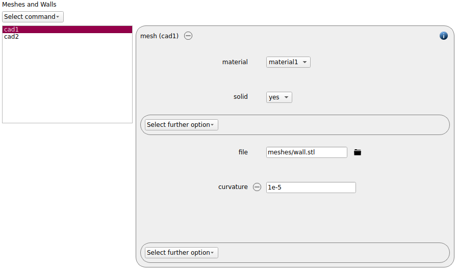
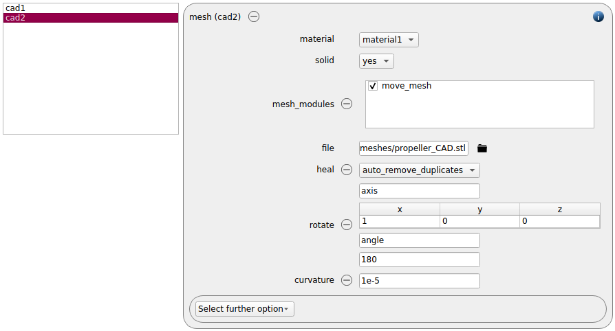
Two meshes that are used as geometries:

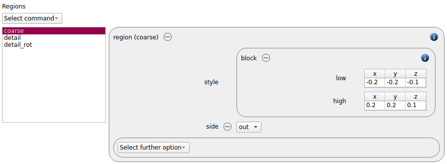
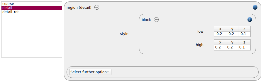
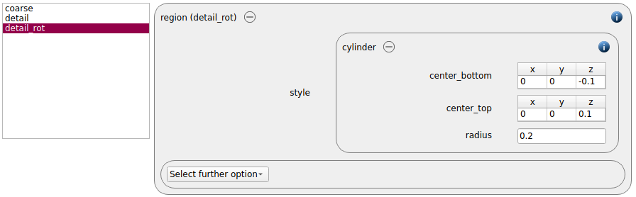
We define three different regions. The two regions coarse and detail do not intersect and their union covers the simulation domain. The third region detail_rot defines the cylindric region for the MRF zone. The region coarse is used for applying a classical one-way coupling command with a stationary velocity field. The other two zones are used for the one-way coupling command with the moving reference frame, i.e., the command with the rotating velocity field zone.

Physics models

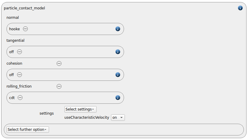
The contact models are now defined. For the particles we use the normal contact model hooke and the rolling friction model cdt.

Since we added a mesh in the previous section, a wall contact model is also added automatically to this section. We use the normal model hooke:

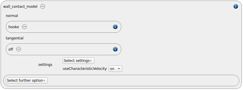
In both cases the hooke model is used with the setting useCharacteristicVelocity on.

Finally, the gravity is enabled:

Per default the gravity has a magnitude of 9.807 and acts into negative z-direction. These defaults can be changed by either setting the magnitude or the direction manually.

Particles

In the general settings tab we only defined a single material type (default), whose settings have to be specified here:

	default
Density	400
Young’s modulus	1e7
Poisson’s ratio	0.45
Coefficient of restitution	0.5
Coefficient of friction	0.1
Coefficient of rolling friction	0.068

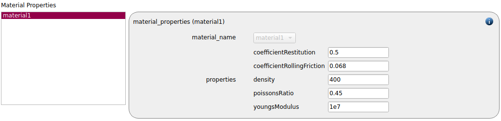
The hooke normal model requires the definition of a characteristic velocity:

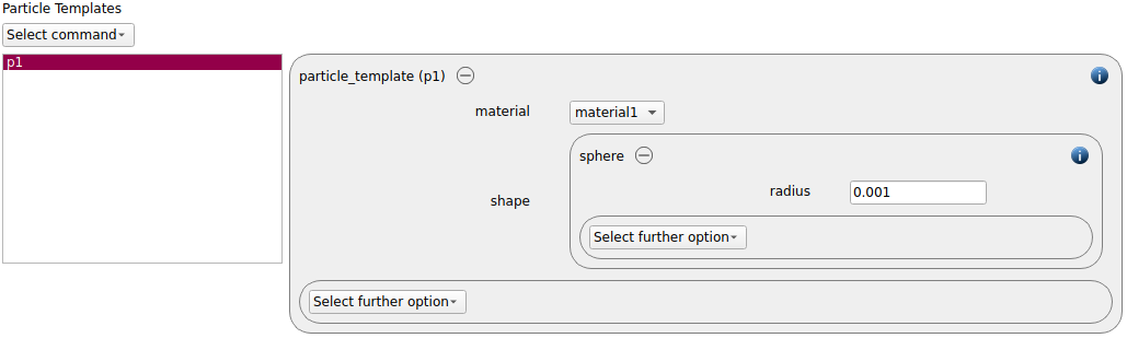
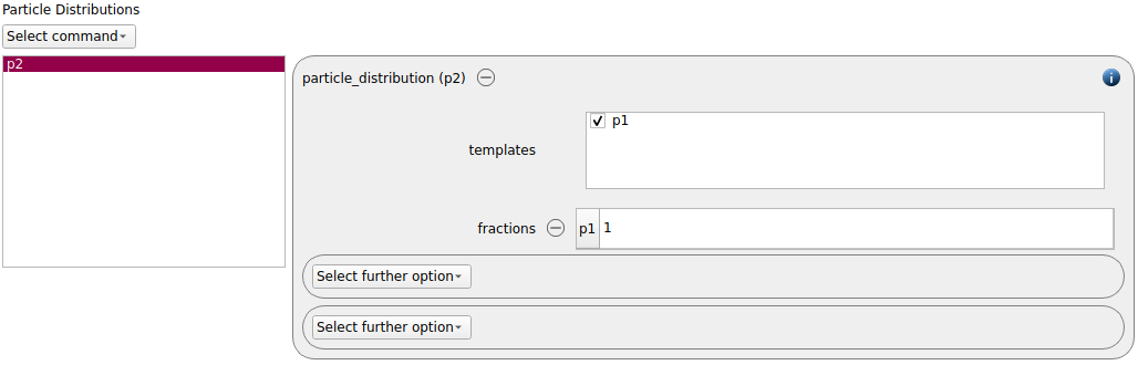
A particle template of style sphere with a radius of 0.001 m is defined and used for a particle distribution:

Particles with a velocity of 0.2 m/s in negative z-direction are inserted using an insertion command command with mode stream:

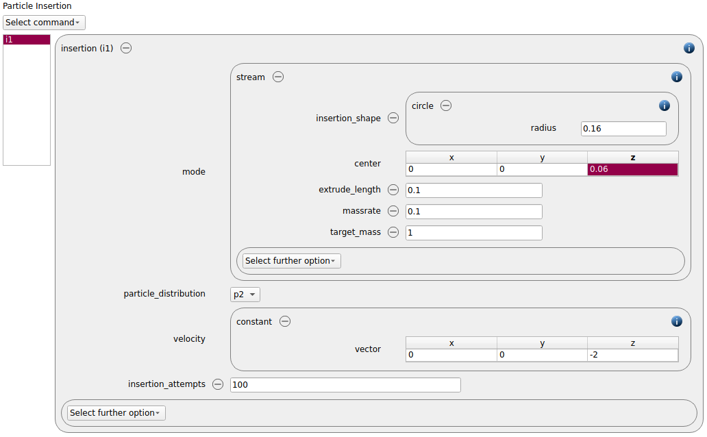
The insertion domain is defined by a generic insertion shape as well as an extrusion length.

Coupled simulation

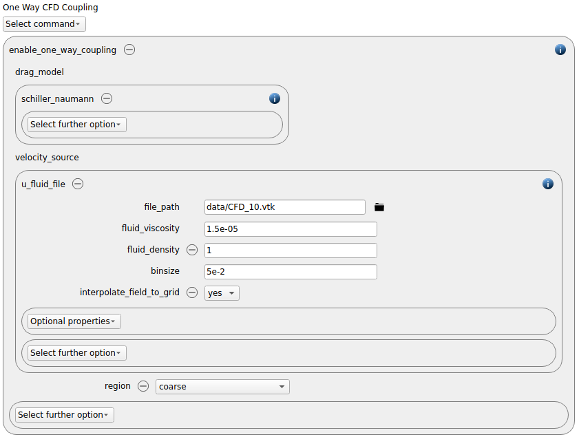
In this tab we define two one-way coupling commands. The first command is applied to the region “coarse” and uses a single fluid velocity field:

The second command is applied to region “detail” and uses a much small bin size. Furthermore a MRF_region keyword is used to define the region for the moving reference frame (i.e., the zone in which the defined velocity rotates at a given rotational velocity).

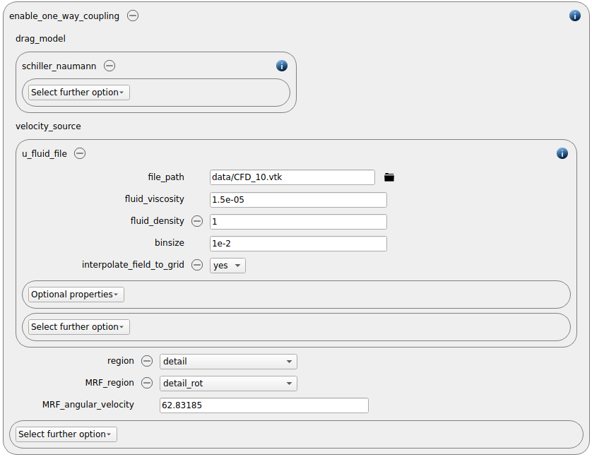
It is always recommended to set the option interpolate_field_to_grid to yes. Otherwise a very strict definition of the velocity fields is required. The file for the velocity field is provided in vtk format.

Simulation control

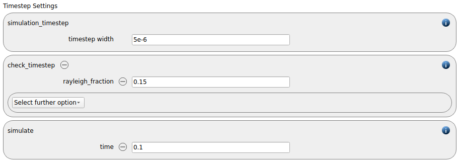
In this tab, we first define the time-step settings such as the desired simulation timestep of 5e-6 seconds and the total simulation time of 0.1 seconds. Per default also the check_timestep command command is enabled, which throws a warning when the time step exceeds 10 % of the Rayleigh or the Hertz time. These thresholds can be changed by setting an alternative value for hertz_fraction or, as is done in this case, for rayleigh_fraction.

In this case, a neighbor list skin size of 0.004 leads to optimal simulation results:

The load balancing command is enabled for most efficient parallelization:

Output settings

In this tab we first define the timestep width for the file and the terminal output:

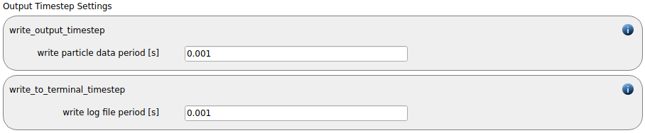
The output_settings command command the takes care that all particle information and the meshes are written to files accordingly. Furthermore it triggers the output of global quantities such as the kinetic energy of the particles or total normal and shear stresses onto meshes to the terminal. Please note that if the output of per-cell information on meshes such as wear, velocity of stress are desired, one has to add the keyword mesh_properties and select the required output.

Running the simulation

After completing the setup and saving it, the simulation can be launched. Hence, change to the Simulation view. First hit the “Check settings” button, and if the check returns “Check settings successfully completed” the simulation can be run by hitting “Start”. Please note that per default the simulation is launched on 4 processors, which can of course be changed depending on your system. If you want to run it serially, please remove the check mark before “Use MPI”.

Postprocessing with Paraview

After the simulation is completed, all data written with the output_settings command can be visualized automatically by going to the Visualization view and hitting the “Start Paraview” button.

The image below shows the particles at the last time step together with both fluid fields that are used by the one-way coupling. The fluid field files are opened manually in Paraview, the representation of the fluid fields is changed to Points. Increasing the point sizes leads to a better visibility. The particle size is scaled up by a factor of 3 for better visibility.