Home
HomeOne way CFD-DEM coupling: using a drag force field
In this tutorial an included fluid velocity field is used to exert a drag force onto particles.
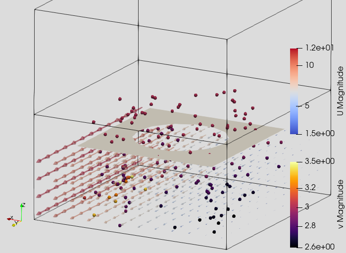
Discussed features are the usage of externally calculated velocity fields as well as their output.
Name of the case: Project_Dragforce_Field
Setting up the simulation
First the used materials command as well as the simulation domain are defined in the General Settings tab. Please note that the dimensions of the simulation domain can only be defined in the first simulation. This means that the box that forms the simulation domain has to be chosen big enough from the beginning.
General settings
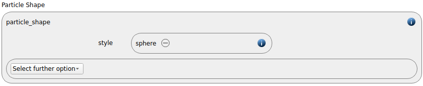
In this simulation we set particles of particle shape sphere:
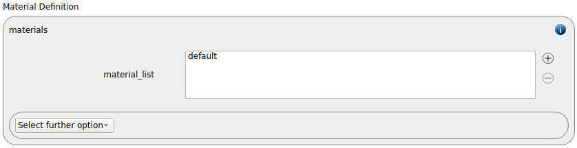
A single materials command with the name default is used:
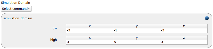
The simulation domain is defined with x dimension ranging from -3 to 3 meters, y dimension ranging from -1 to 5 meters and z domain ranging from -3 to 3 meters.
Meshes and regions
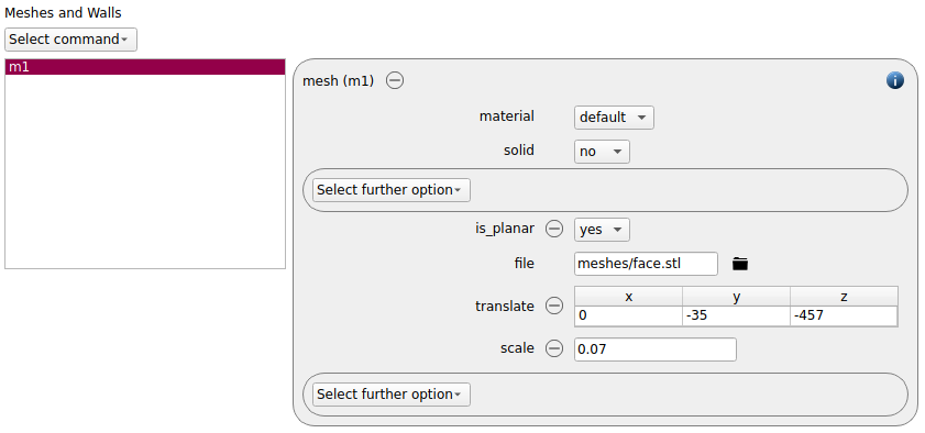
For the particle insertion we will use a mesh command, which is loaded with the options solid no and is_planar yes:
In the next step, a region command called drag is generated:
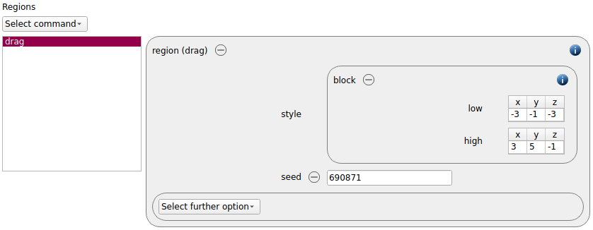
Later on, a drag force will be applied to this region.
Physics models
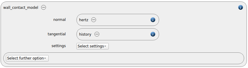
In this step we define the contact models. For the particles we use the normal contact model hertz and the tangential model history.
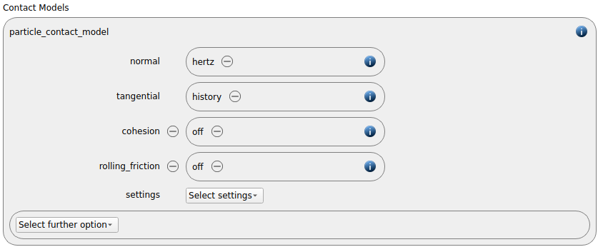
Since we added a mesh in the previous section, a wall contact model is added automatically in this section. As the mesh is not used as wall, the selection of the contact models plays no role here.
In this simulation we do not consider the effect of the gravity force. Therefore, we need to remove the automatically added gravity term from the body forces section:

Particles
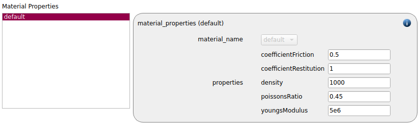
In the general settings tab we only defined a single material type (default), whose settings have to be specified here:
default |
|
Density |
1000 |
Young’s modulus |
5e6 |
Poisson’s ratio |
0.45 |
Coefficient of restitution |
1 |
Coefficient of friction |
0.5 |
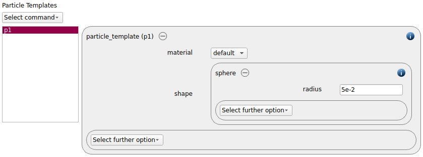
A particle template with spheres of radius 0.05 m and of the defined material is generated:
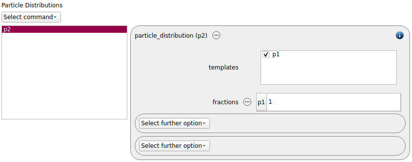
The template is used to create a particle distribution as follows:
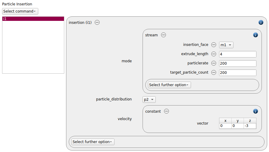
The final step in the tab is the definition of the insertion. An insertion command command with mode stream is used to insert 200 particles at a rate of 200 particles/second. The initial velocity of the particles is given with (0,0,-3) m/s, the orientation is set to random. The previously loaded mesh is used as insertion face with an extrude length of 4. Furthermore, the overlap check is set to yes (this is the default value), all_in is set to no.
Coupled simulation
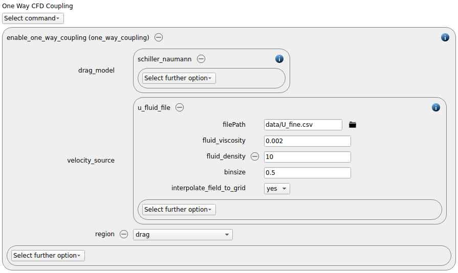
In the next step the definition of the drag force field takes place. The command enable_one_way_coupling command is used with a Schiller Naumann model. The fluid viscosity is set to 0.002 m^2/s and the density to 10 kg/m^3. The binsize is set to 0.5 meters and the interpolate option is set to yes:
Simulation control
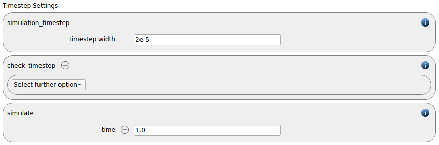
In this tab one first choses the time step settings such as the desired simulation timestep of 2e-5 seconds and the total simulation time of 1.0 second. Per default also the check_timestep command command is enabled, which throws a warning when the time step exceeds 10 % of the Rayleigh or the Hertz time. These thresholds can be changed by setting an alternative value for hertz_fraction or rayleigh_fraction.
Output settings
In this tab we first define the timestep width for the file and the terminal output:
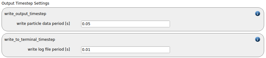
The output_settings command command the takes care that all particle information and the meshes are written to files accordingly. Furthermore it triggers the output of global quantities such as the kinetic energy of the particles or total normal and shear stresses onto meshes in the terminal. Please note that if the output of per-cell information on meshes such as wear, velocity of stress are desired, one has to add the keyword mesh_properties and select the required output.

Running the simulation
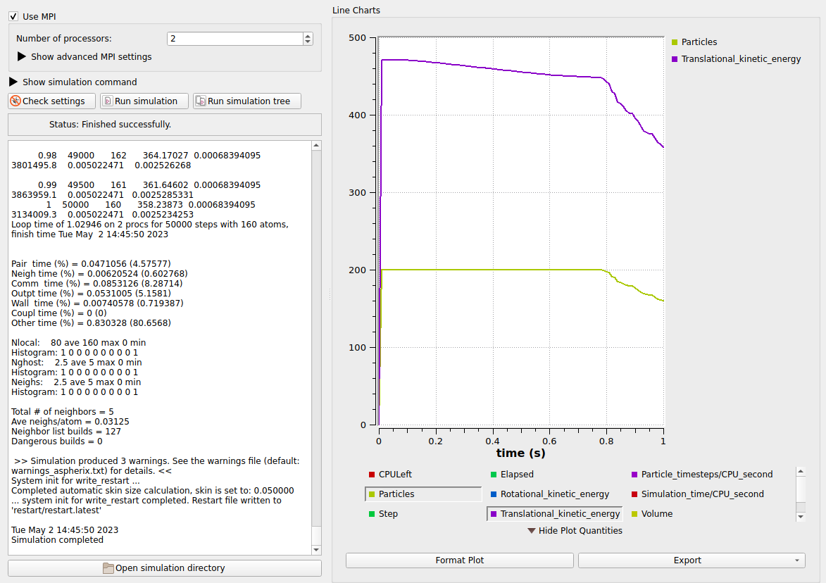
After completing the setup and saving it, the simulation can be launched. Therefore change to the Simulation view. First hit the “Check settings” button, and if the check returns “Check settings successfully completed” the simulation can be run by hitting “Start”:
Postprocessing with Paraview
After the simulation is completed, all data written with the output_settings command can be visualized automatically by going to the Visualization view and hitting the “Start Paraview” button.
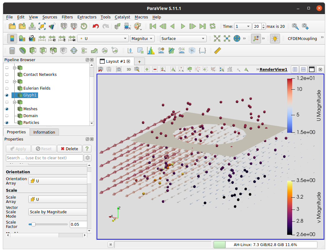
The Eulerian field that is generated by the enable_one_way_coupling command is also loaded. For a better visualization one could for example apply an opacity to it:
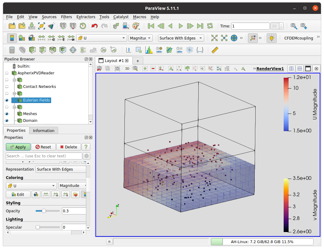
For displaying the velocity field as a field of vectors, one can use a glyph filter. By setting both the orientation and the scaling vector to U, one gets the velocity vector field with vectors scaled according to the velocity magitude. Please use an appropriate scaling factor (here 0.05) for a good representation: