Radiation using distance based approximations

This tutorial case demonstrates how to set up a case with radiative heat transfer using the distance based approximation method. This method relies on using a view-factors file that accounts for how much radiated heat each particle sees depending on distance from the heat source and the void fraction.

Name of the case: Project_Radiation

Simulation setup

The case consists of a simple setup with a heater mesh that will radiate to the particles falling in front of it.

General settings

In the General Settings tab particle shape, materials and simulation domain are defined.

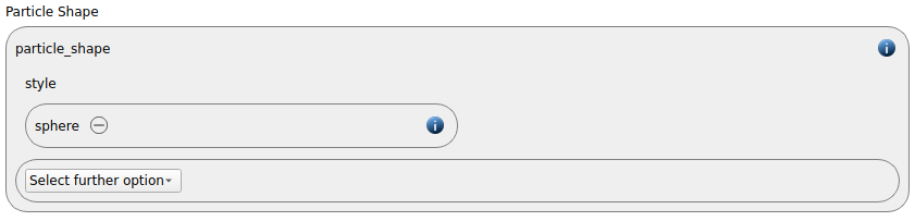
We start with setting the particle shape type to sphere:

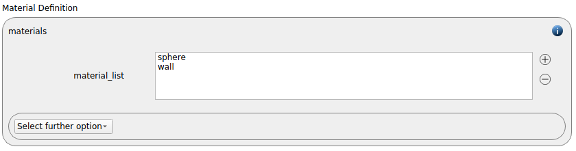
We use two materials command, one for walls and another for the particles:

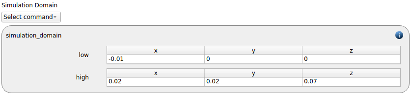
The simulation domain is defined with the following dimensions:

	min	max
x	-0.01	0.02
y	0.0	0.02
z	0.0	0.07

Meshes and regions

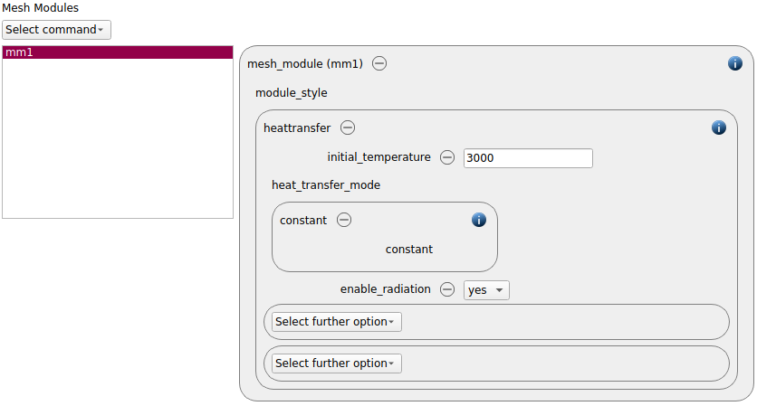
The heater will need a mesh module for heat transfer to work as the heat source for radiation. We set this up first in the Mesh Module settings. Heat transfer mode is constant and the initial mesh temperature is set to 3000 K. The keyword enable_radiation sets this as a radiation source:

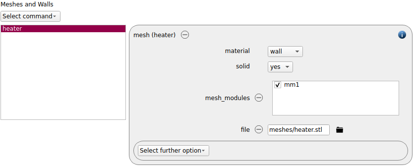
We then use a prepared geometry (stl file) as mesh command for the heater. Note the loaded mesh module:

Physics models

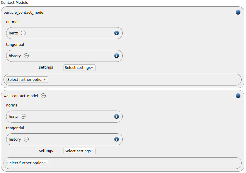
In this tab we set contact models and other physical models. Both particle_contact_model command and wall_contact_model command are set to the normal model hertz and the tangential model history:

The gravity command is added automatically:

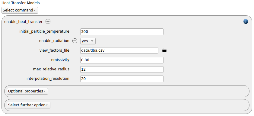
We also enable heat transfer for modelling radiation with the enable_heat_transfer command command. Here we define the view factors file for the DBA method, the emissivity of the particles and the max_relative_radius used as cut-off distance for calculating radiation:

Particles

In this section one sets the material related parameters and defines all particle templates, particle distributions and insertion commands.

All parameters required by contact models and other physical models in the simulation are automatically added as material properties. In this case, we need to set the properties for both materials:

Parameter	sphere	walls
Coefficient of friction	0.72	0.5
Coefficient of restitution	0.82	0.44
Density	1000	1000
Poissons ratio	0.3	0.3
Youngs modulus	1e9	1e9
Thermal capacity	1	1
Thermal conductivity	0	0

Setting thermal conductivity to 0 disables heat conduction, making sure the case is dealing only with radiation. This way, particles won’t heat up due to collisions with other particles or the walls.

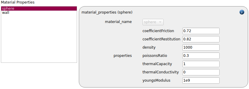
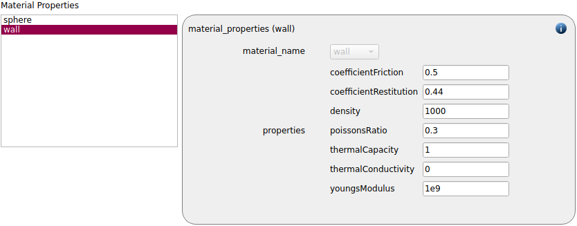
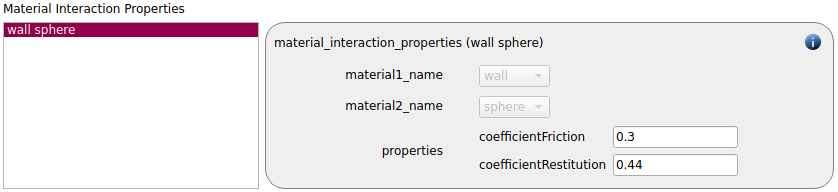
Since we have two materials, we need to define material interaction properties:

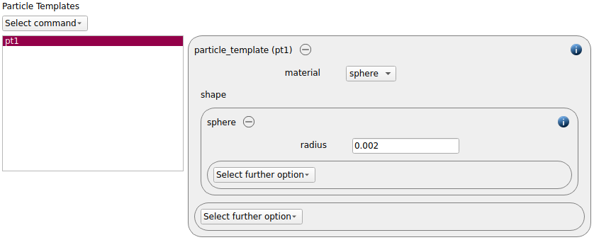
A particle template for spheres with a radius of 2 mm is generated:

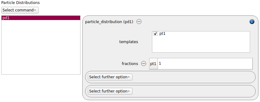
This template is used to define a particle distribution:

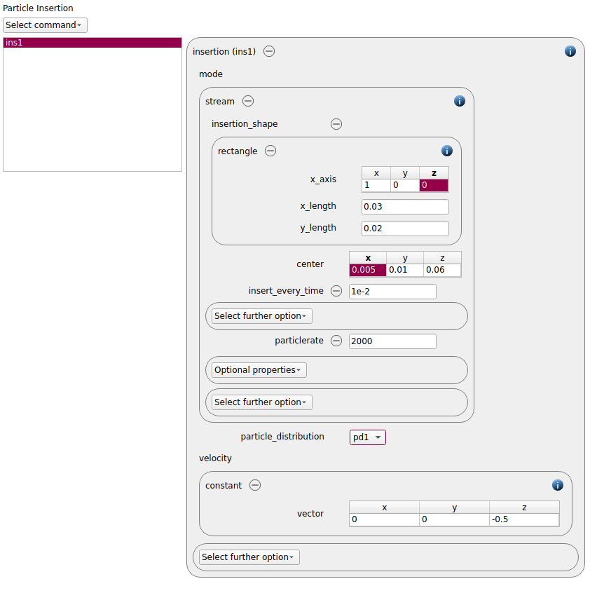
After generating the distribution, a way to insert the particles has to be selected. An insertion command command with the mode stream is used for continuous particle generation with a particle rate of 2000 particles per second. The initial velocity of the particles is set to (0 0 -0.5) m/s. The particles are inserted via a rectangular shape:

Simulation control

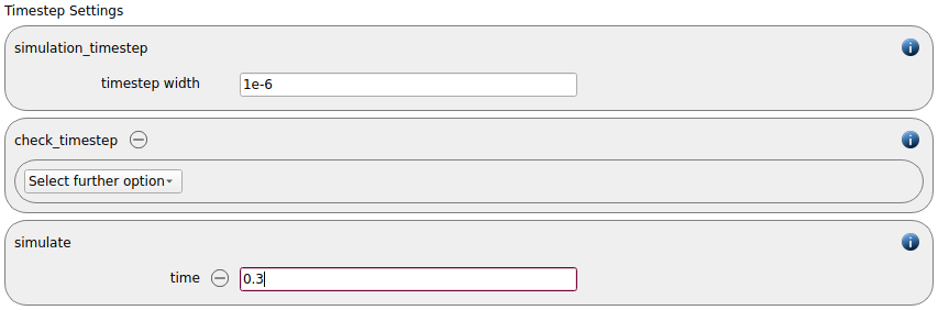
We define the time step settings simulation timestep of 1e-6 seconds and the total simulation time of 0.3 seconds. Per default also the check_timestep command command is enabled, which throws a warning when the time step exceeds 10 % of the Rayleigh or the Hertz timestep. These thresholds can be changed by setting an alternative value for hertz_fraction or rayleigh_fraction.

We also enable neighbor_optimization in the neighbor list settings, which helps with the radiation calculation:

Output settings

We first define the time between each file and terminal output:

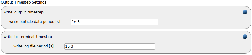
The “output_settings” command the takes care that all particle information and the meshes are written to files accordingly. Furthermore it triggers the output of global quantities such as the kinetic energy of the particles or total normal and shear stresses onto meshes in the terminal.

We keep the default output_settings command:

The setup of this case is now complete, we can save the setup and move on to the simulate section.

Running the case

You can now press the Run button in the Simulations tab. While the simulation is running, you can check output in the log or check the plots for various simulations quantities. The number of particles in the simulation over time is shown below:

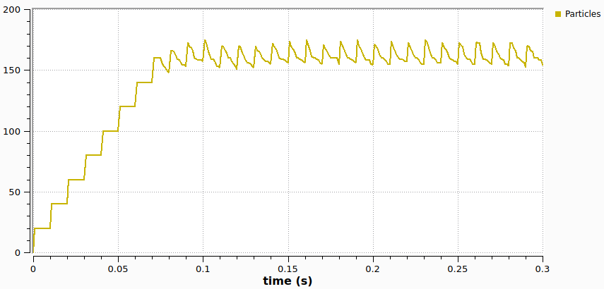
The data displayed in the graph can be edited and saved as image for further usage in reports and presentations.

Postprocessing

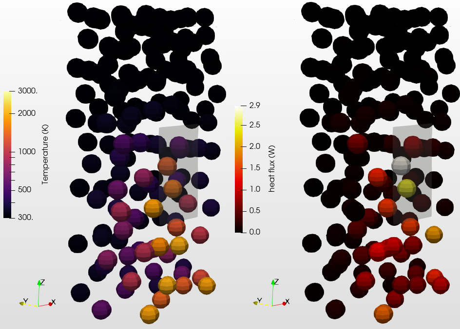
As soon as data was written to the post folder within the simulation, it can be displayed with Paraview or Ovito. The image below shows particle temperature and heat flux visualized in Paraview: