Spray modelling with DEM spray particles

This tutorial shows the simulation of spray-coating particles with a liquid that is modelled by DEM spray particles. The spray is generated with a conical nozzle and causes the formation of a liquid film both on the particles and the wall area in the spraying zone.

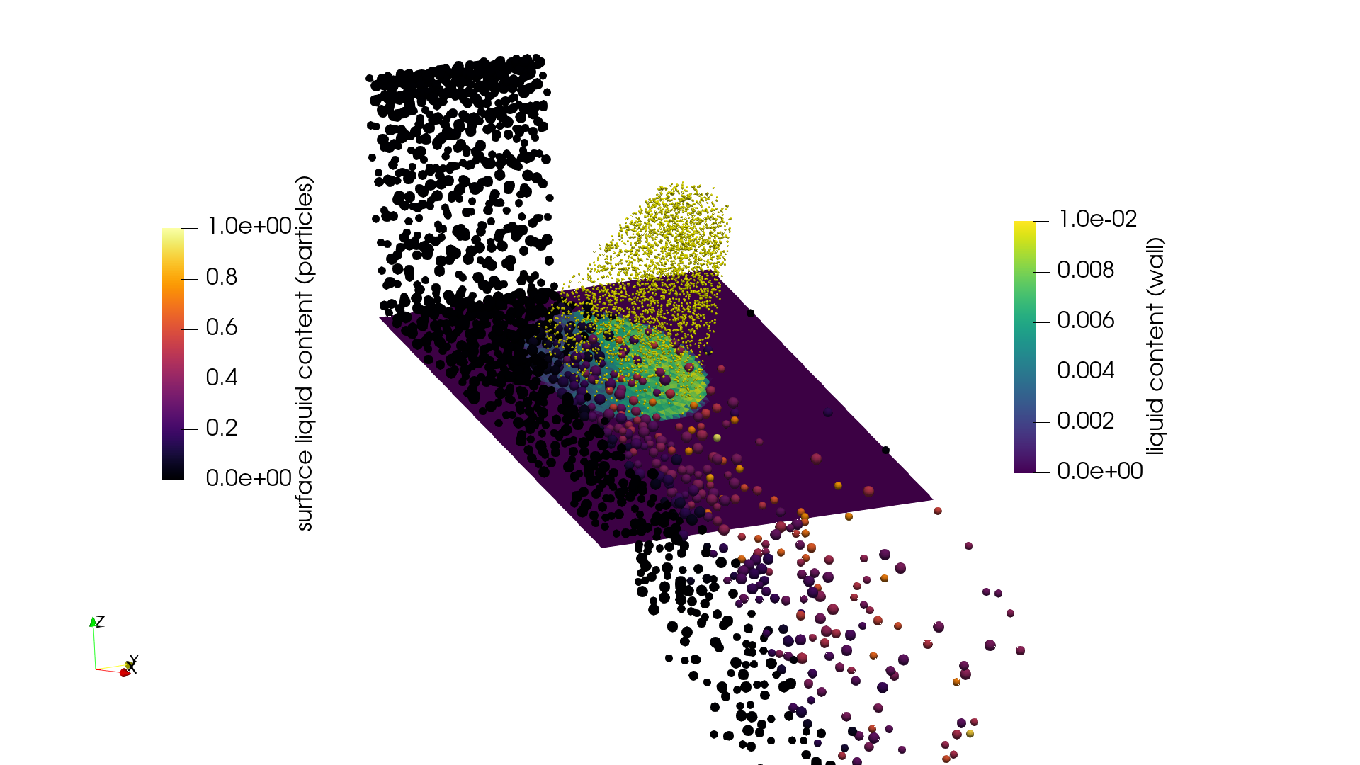
The image shows the solid particles and the backplate colored with respect to the surface liquid content.

Name of the case: Project_Lagrangian_Spray_Modelling

Setting up the simulation

As a first step, the particle shape, the used materials command and the simulation domain are defined in the General Settings tab.

General settings

In this simulation we set particles of particle shape sphere:

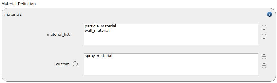
Two regular materials command “particle_material” and “wall_material” and a single custom material “spray_material” are generated:

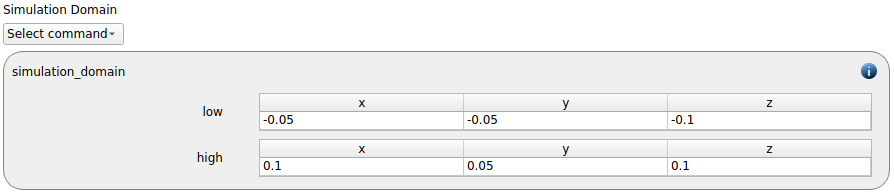
The simulation domain ranging from -0.05 to 0.1 in x, from -0.05 to 0.05 in y and from -0.1 to 0.1 in z direction is created:

Meshes and regions

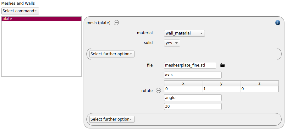
For the backplate, a mesh command is inserted. It consists of wall_material and is inclined by an angle of 30 degrees around the y-axis:

Physics models

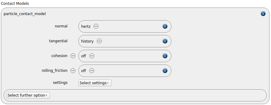
The contact models are now defined. For the particles we use the normal contact model hertz and the tangential model history.

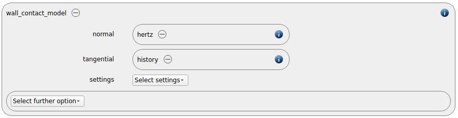
Since we added a mesh in the previous section, a wall contact model is also added automatically to this section. We use the default models normal hertz and tangential history:

The gravity is enabled automtially:

Per default the gravity has a magnitude of 9.807 and acts into negative z-direction. These defaults can be changed by either setting the magnitude or the direction manually.

To enable spray modelling, the liquidtranport command has to be added:

Particles

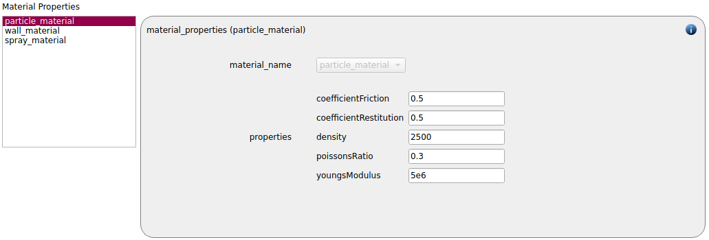
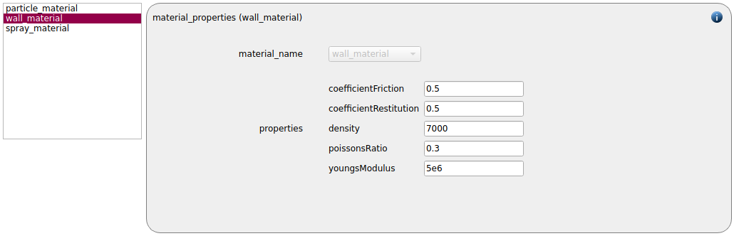
In the general settings tab the material properties for the particle_material and the wall_material are specified:

	particle_material	wall_material
Density	2500	7000
Young’s modulus	5e6	5e6
Poisson’s ratio	0.3	0.3
Coefficient of restitution	0.5	0.5
Coefficient of friction	0.5	0.5

For the spray_material, the custom material properties are required:

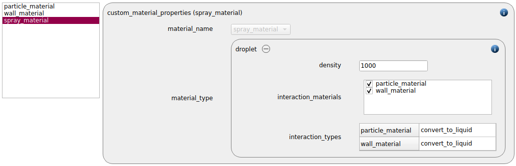
In this case, the spray particles will be converted to liquid, both when they hit the backplate or a solid particle.

Since two solid materials are present, also the material interaction properties must be set:

	wall_material - particle_material
Coefficient of friction	0.5
Coefficient of restitution	0.5

The liquid transport model requires the definition of the initial liquid content:

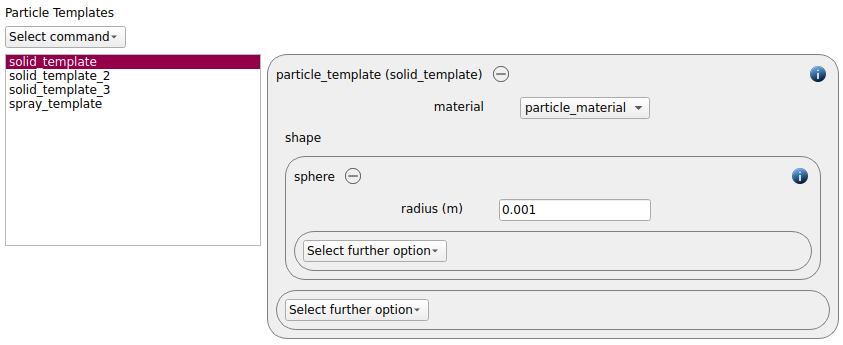
For the solid phase, three particle templates solid_template_1, solid_template_2 and solid_template_3 of shape sphere with radii of 0.001, 0.0012 and 0.0014 are added:

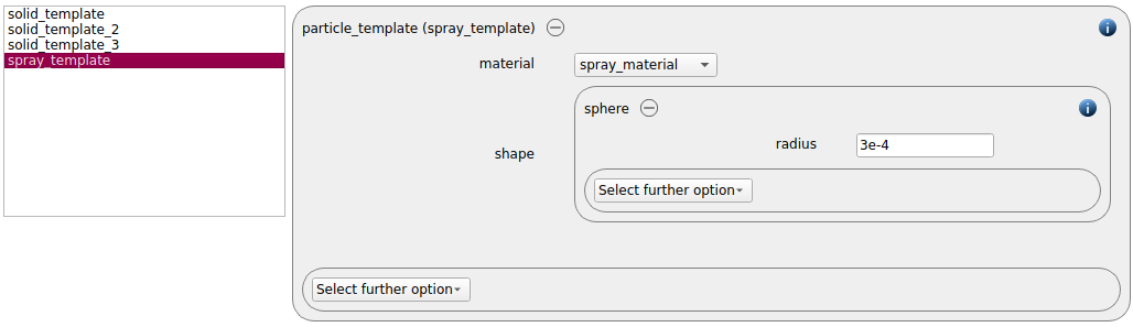
For the spray particles a particle template of shape sphere with a radius of 3e-4 is added:

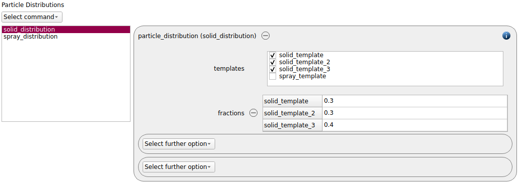
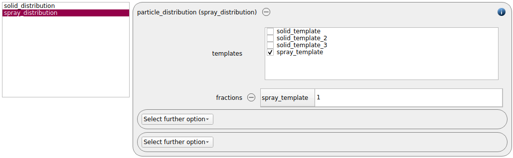
The particles templates are used for two different particle distributions:

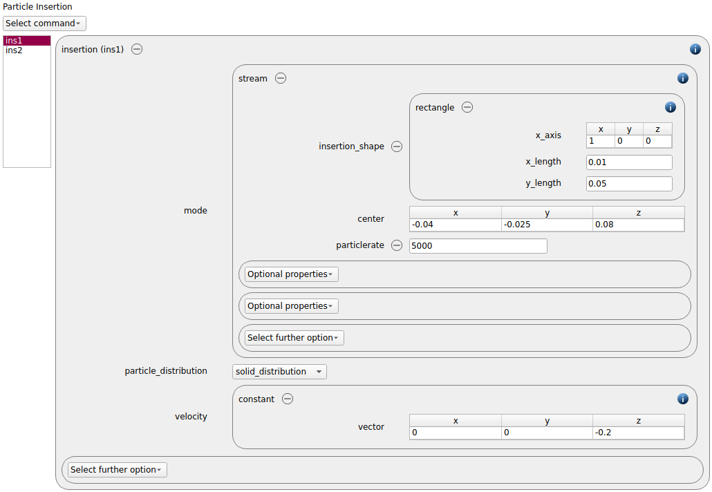
Two insertion command commands are used for the insertion of solid and spray particles. For the solid particles, a command of type stream is applied. The particles are inserted through a rectangular insertion shape with a center of (-0.04, -0.025, 0.08), an x-length of 0.01 and a y-length of 0.05 meters. The insertion velocity is -0.2 m/s in negative z-direction and a particle rate of 5000 particles per second is used:

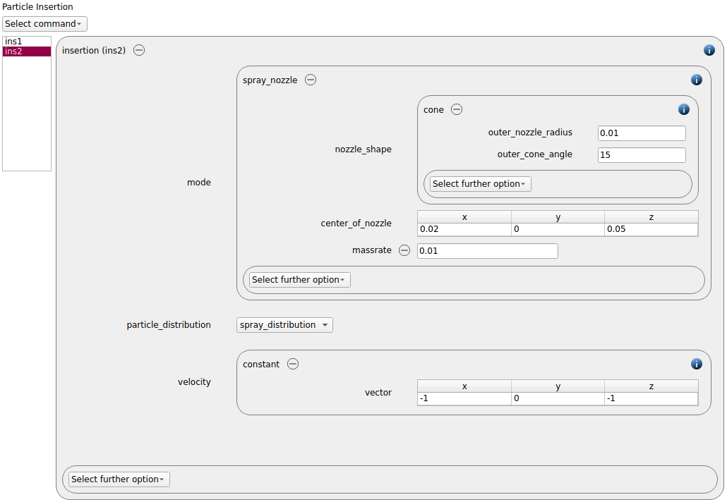
For the generation of the spray we use an insertion command of type spray_nozzle. A concical spray nozzle with an outer radius of 0.01 meters and an outer cone angle of 15 degrees is created at the center (0.02, 0, 0.05). The liquid is inserted with a velocity of (-1, 0, -1) m/s and a massrate of 0.01 kg/s:

Simulation control

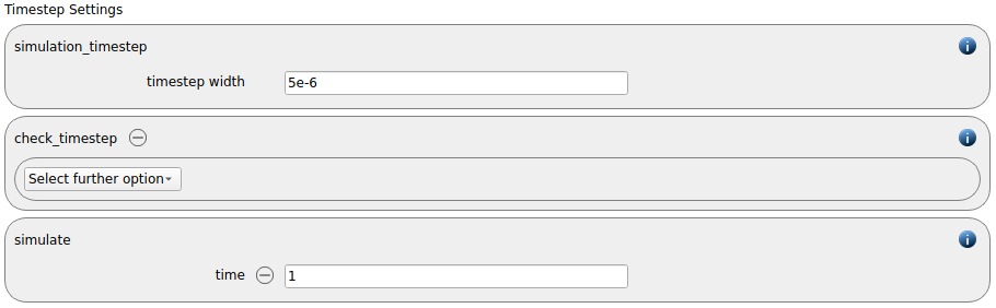
In this tab, we first define the time-step settings such as the desired simulation timestep of 5e-6 seconds and the total simulation time of 1 second. Per default also the check_timestep command command is enabled, which throws a warning when the time step exceeds 10 % of the Rayleigh or the Hertz time. These thresholds can be changed by setting an alternative value for hertz_fraction or rayleigh_fraction.

Loadbalancing is enabled per default:

Output settings

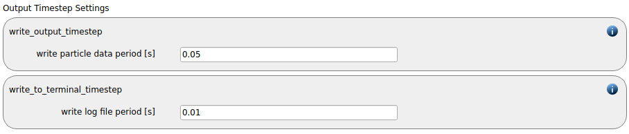
In this tab we first define the timestep width for the file and the terminal output:

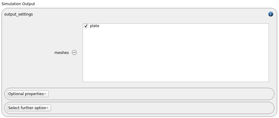
The output_settings command command the takes care that all particle information and the meshes are written to files accordingly. Furthermore it triggers the output of global quantities such as the kinetic energy of the particles or total normal and shear stresses onto meshes to the terminal. Please note that if the output of per-cell information on meshes such as wear, velocity of stress are desired, one has to add the keyword mesh_properties and select the required output. If one or more meshes are added to the meshes list but no mesh properties are selected, all available properties are added to the output, we therefore add the plate mesh to the meshes list:

Running the simulation

After completing the setup and saving it, the simulation can be launched. Change to the Simulation view and set the number of cores to use to 2. Please note that using more cores would rather increase the simulation times instead of decreasing them due to the low number of particles in the simulation. First hit the “Check settings” button, and if the check returns “Check settings successfully completed” the simulation can be run by hitting “Start”.

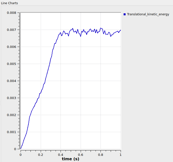
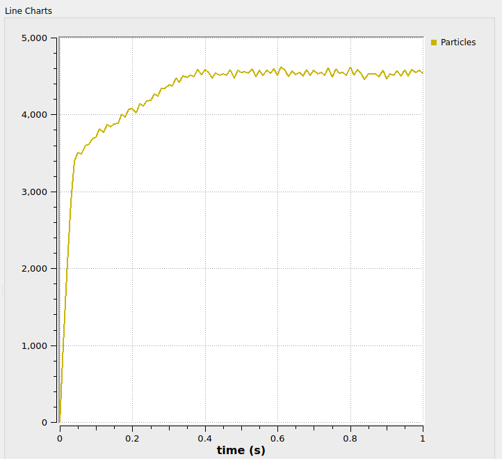
The graphs below shows the kinetic energy and the number of particles as a function of time:

Postprocessing with Paraview

After the simulation is completed, all data written with the output_settings command can be visualized automatically by going to the Visualization view and hitting the “Start Paraview” button.

The image below shows the final state of the system: