Heat transport and evaporation

In this tutorial we show the effect of a temperature field onto a dry and a wet particle that moves through a box at constant velocity. We combine the heat transfer model with the one-way CFD coupling command (fluid velocity and temperature), for the wet particle a liquid transfer evaporation model is used. The results can be validated against theoretically obtained results (in our case with octave):

Name of the case: Project_Heat_Transfer_Evaporation

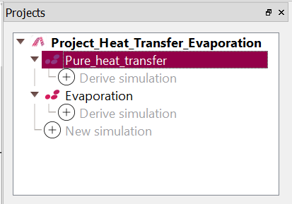
We start with creating a project with two simulations at the same level:

Heat Transfer in the Presence of a Fluid Temperature Field

General settings

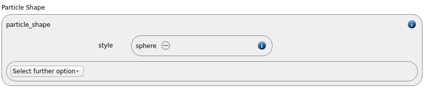
We start with selecting “sphere” as particle shape:

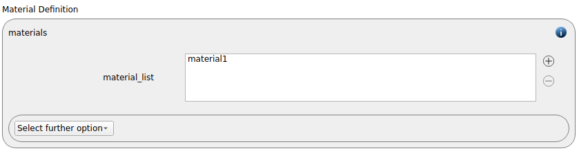
We keep the default entry for the material

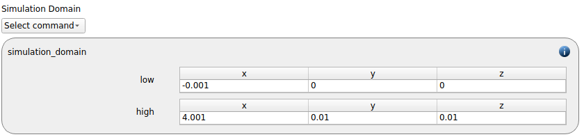
and create a simulation domain that reaches from -0.001 to 4.001 in x-direction and from 0 to 0.01 in y and z-direction:

Meshes and regions

For the current case no changes are required in this section:

Physics models

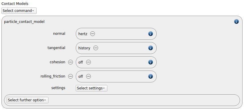
We use the standard contact model normal hertz and tangential history:

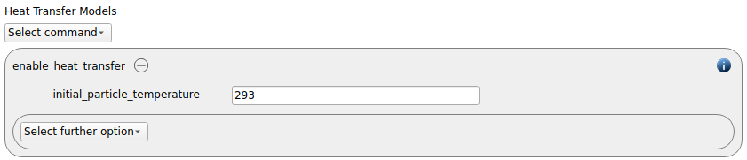
The heat transfer model is switched on with an initial particle temperature of 293 degrees.

The gravity is not considered, so the default enable_gravity command command is removed.

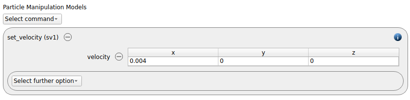
For obtaining a constant particle velocity throughout the whole simulation, we use a set_velocity command command from the Particle Manipulation Models section. In x-direction we prescribe a velocity of 0.004 m/s, in y and z-direction a velocity of 0 m/s.

Particles

We set the material_properties command for the particle material:

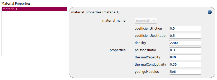
The particle has a density of 2200 kg/m^3, the Young’s modulus is set to 5e6, the Poissons ratio is given with 0.3, the coefficients of restitution and friction with 0.5. The parameters required for the heat transfer were added automatically when selecting enable_heat_transfer, the thermal conductivity is set to 0.35 and the thermal capacity to 840.

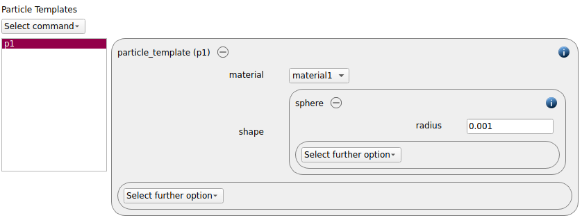
A spherical particle template with a radius of 0.001 is generated:

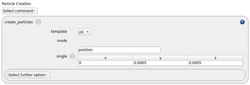
The create_particles command command is used to create a single particle at the beginning of the box at the coordinates 0,0.0005 0.0005:

Coupled simulation

The one-way CFD coupling is achieved by using the enable_one_way_coupling command command:

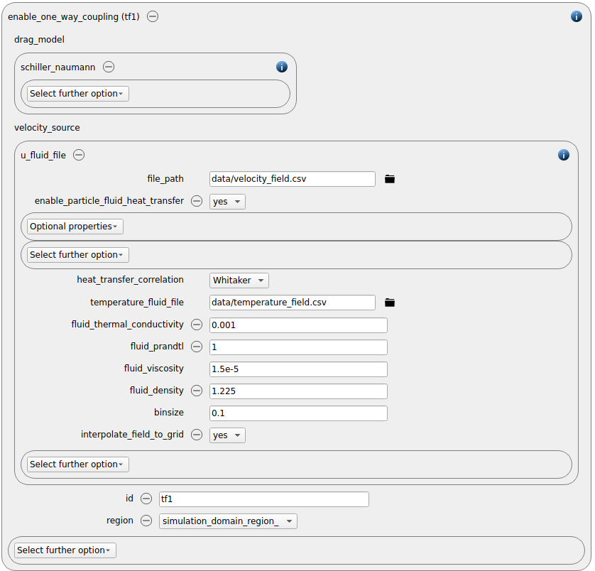
The velocity field is 0 everywhere, and has the form

x y z U_x U_y U_z
0 0.005 0.005 0 0 0
4 0.005 0.005 0 0 0

The temperature field is defined by a line of grid points with a distance of 0.1 m from x = 0 to x = 4 with values decaying linearly from 600 to 350 K.

x y z T
0 0.005 0.005 600
0.1 0.005 0.005 593.75
0.2 0.005 0.005 587.5
.
.
.
3.8 0.005 0.005 362.5
3.9 0.005 0.005 356.25
4 0.005 0.005 350

It is generally recommended to use the keyword “interpolate_field_to_grid” at all times, it makes the whole command a lot more stable. However, please note that the algorithm still requires sufficient temperature / fluid information. It will, for example, no use a linear interpolation between two points at the beginning and the end of the domain. Please make sure that the distance of the points is somewhere in the range of the binsize.

Simulation control

In the next section we define the simulation time step and the total simulation time:

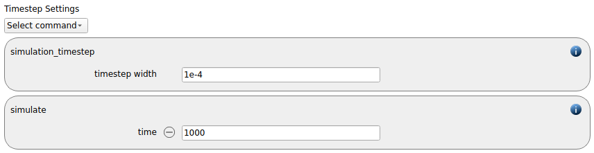
Since the particle motion is prescribed and not evaluated directly, and since heat transfer is a relatively slow process, it is possible to use a relatively large time step here. The check_timestep command command calculates the Rayleigh and Hertz timestep fraction, which play no role in this case - the entry can thus be removed.

Output settings

Due to the long simulation time of 1000 seconds we chose an output timestep of 10 seconds and a terminal timestep of 0.1 seconds:

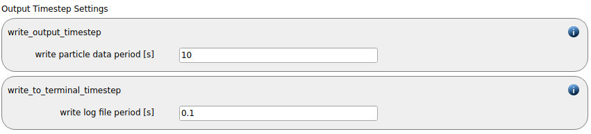
The default output_settings command command is used:

Custom settings

For being able to visualize the temperature, x-position and x-velocity of the particle over time, we add three variables with weight 22 and use them as an input to the status_style command command that gets weight 24:

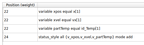
Please note that the particle temperature variable accesses the internally created “Temp” field. The length of all the accessed fields corresponds with the number of particles in the simulation. Since in this case only a single particle is present, accessing the value for the particles with id 1 yields the desired values.

It is important that the weight of the status style command is higher than the weight of the output_settings command (23), since it overwrites some of its settings. The weight must, after all, also be lower than the weight of the simulate command (26).

Simulation and results

This was the last setting in for this calculation. Please save the project and change to the Simulation tab. Uncheck the box before “Use MPI” - for a single particle a serial calculation is sufficient. After running the simulation the following curve for the particle temperature shows:

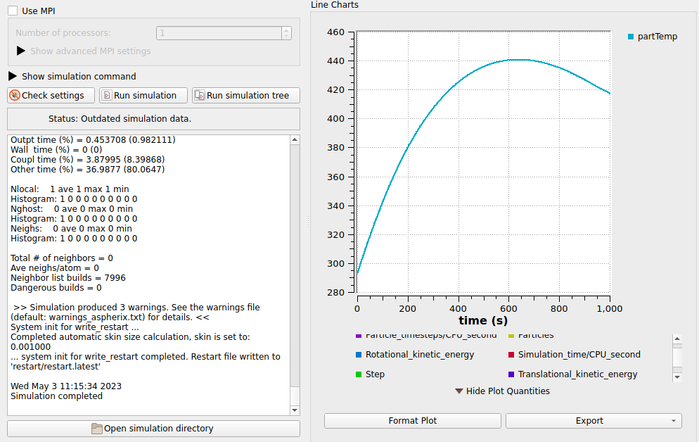
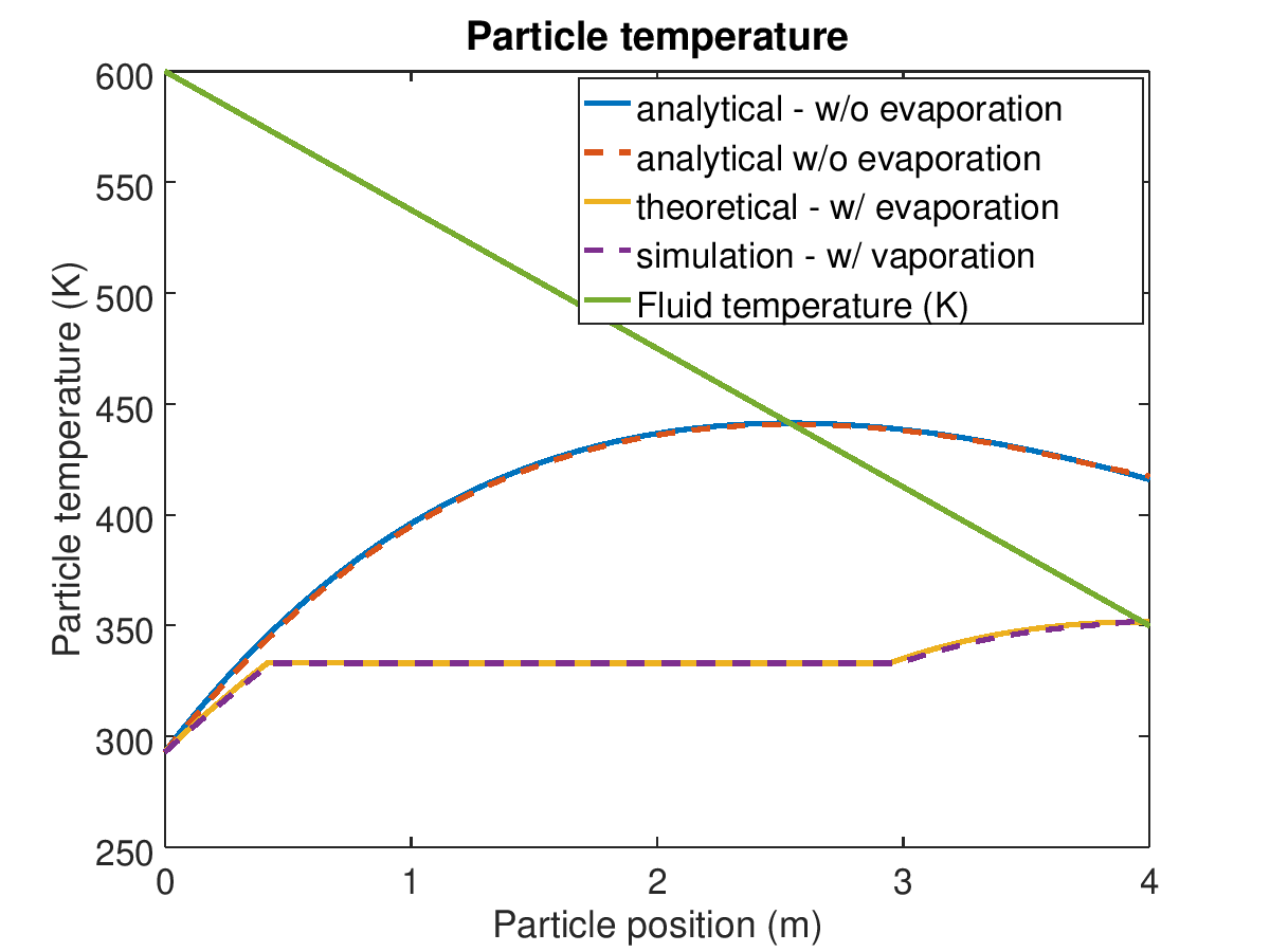
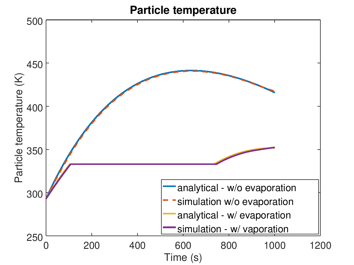
The curve reflects the fact the particle moves through a domain with decaying temperature. First it gets heated up strongly, until it becomes hotter than the fluid region it starts to pass. Consequently, the particle temperature starts to decrease then again.

Heat Transfer and Evaporation in the Presence of a Fluid Temperature Field

The setup of this case is similar to the case setup of the previously presented heat transfer case. Make a copy of the previously defined case and rename it to “Evaporation”. Then move on to the Physics models tab.

Physics models

There, we add a liquid transport model with the keyword evaporation:

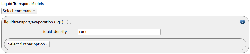
The fluid density is set to 1000 kg/m^3.

Particles

The addition of the liquidtransfer model leads to more keywords in the material properties section, namely the evaporation temperature, the latent heat and the liquid heat capacity:

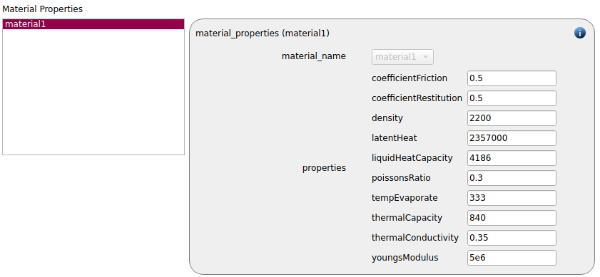
Furthermore a global scalar for the initial surface liquid content is added:

Custom settings

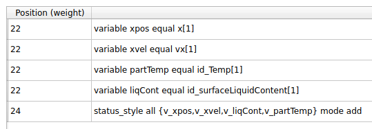
In order to see the temperature of the particle and its surface liquid content we define variables that contain these values. The internal name of the particle temperature field is Temp, the name of the surface liquid content field is surfaceLiquidContent. These fields have one entry per particle, and since only a single particle is present in the simulation, we can be sure the obtain the right value when accessing the values of the particles with id one.

Furthermore the x-position and the x-component of the velocity of the particle should be visualized, thus we also define variables for accessing them. The status_style command command is used to replace the “classical terminal output” that is triggered by the output_settings command with the customized output quantites.

Please note that the variables time, step, atoms and ke (kinetic energy) are global variables that are defined within Aspherix and that can be used directly. Custom variables are accessed by adding prepending “v_” to their name.

Simulation and results

With this last setting the case setup is completed. Please remove the check mark in front of the “Use MPI” check box - a serial run is completely sufficient for this case. In the results graph, both the particle temperature over time and the particle’s liquid content can be displayed:

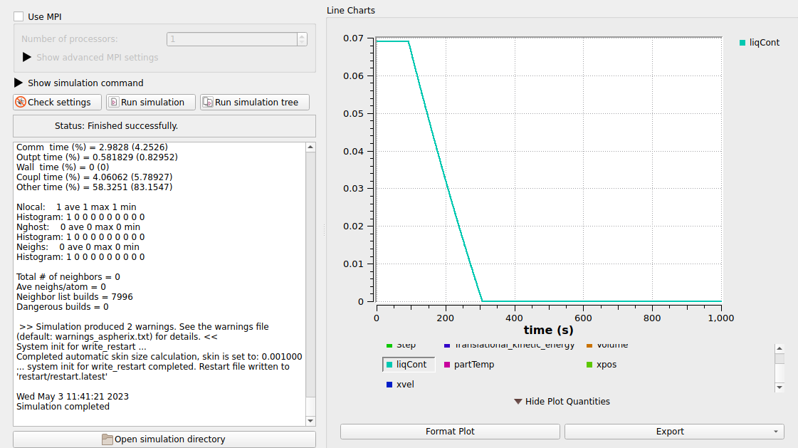
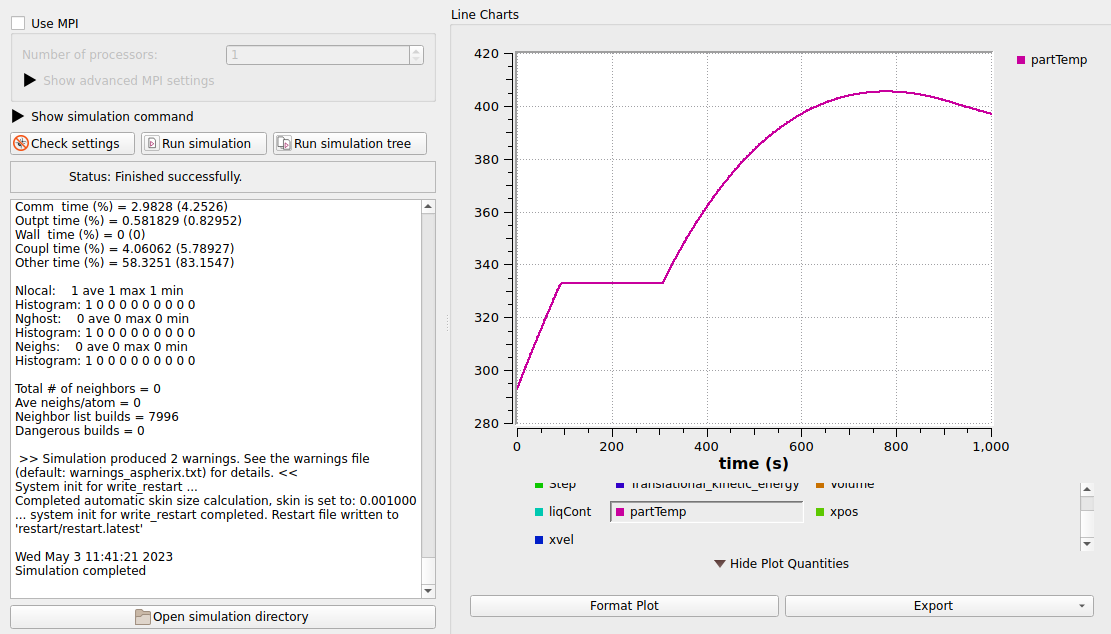
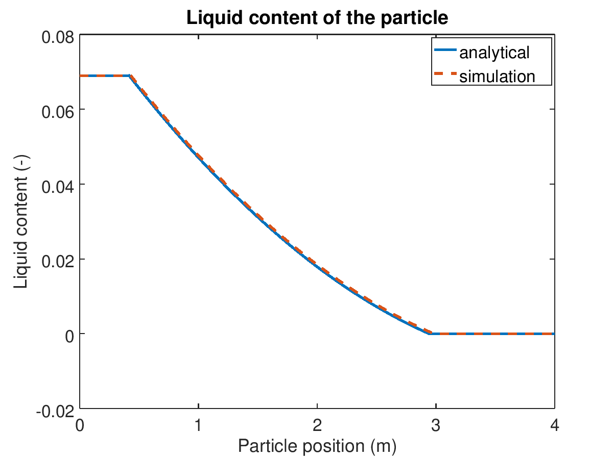
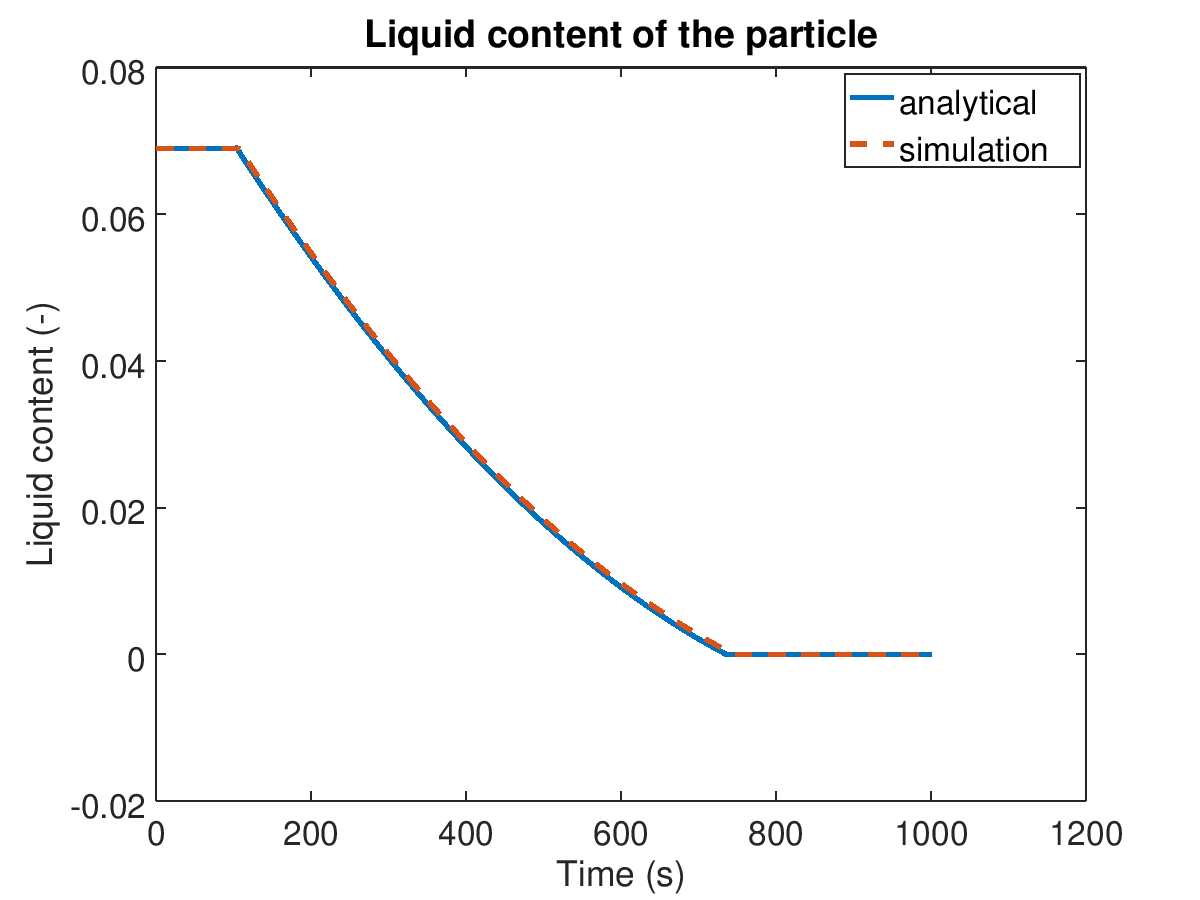
Both graphs reflect the impact of the evaporation: as long as the particle temperature is lower than the evaporation temperature, the particle heats up. When the particle reaches the evaporation temperature, the surface liquid content starts to decrease, the particles starts to dry. Once all liquid has evaporated, the temperature increase of the particle continues.

Validation of the results

For validating the heat transfer with and without evaporation we implmented the following algorithm in octave and compred the results against the simulation results of the presented case:

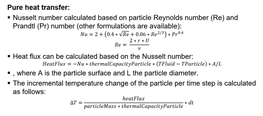
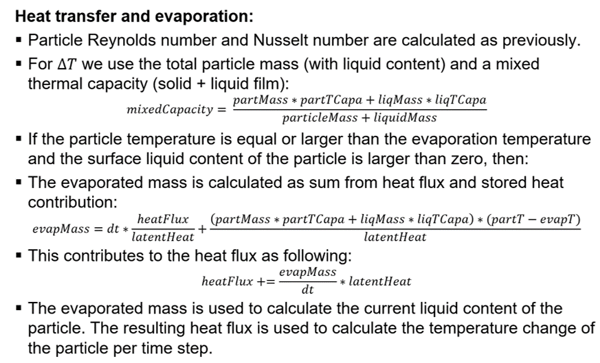
These graphs show that the analytical results and the simulation results match exactly: