Solidification of liquid bridges

This tutorial shows how to simulate the solidification of liquid bridges between particles, and compares the result of the simulation to a case where no solidification takes place.

Both cases consist of two simulations. In the first one a packing of spheres is generated inside a drum geometry. In the second one the drum starts to rotate, and a liquid spray is applied to the particles.

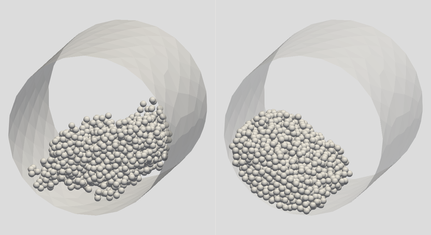
The image below compares the results with solidification (left) and without (right).

Name of the case: Project_Solidification

Simulation 1: Filling

General settings

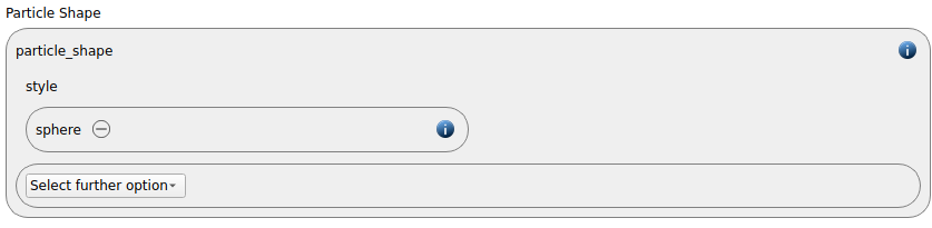
We start with selecting “sphere” as particle shape:

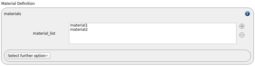
We use two materials (one for the wall, one for the particles):

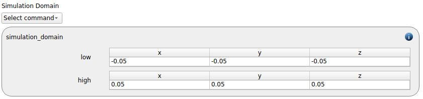
and create a simulation domain that reaches from -0.05 to 0.05 in all three dimensions.

Meshes and regions

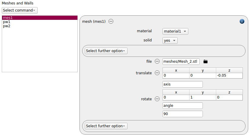
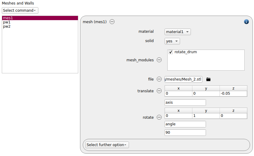
For the drum geometry we import a cylindric mesh command and assign materia1 to it. The mesh must be translated by 0.05 meters in z direction and rotated by and angle of 90 degrees around the y-axis:

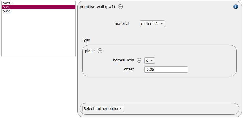
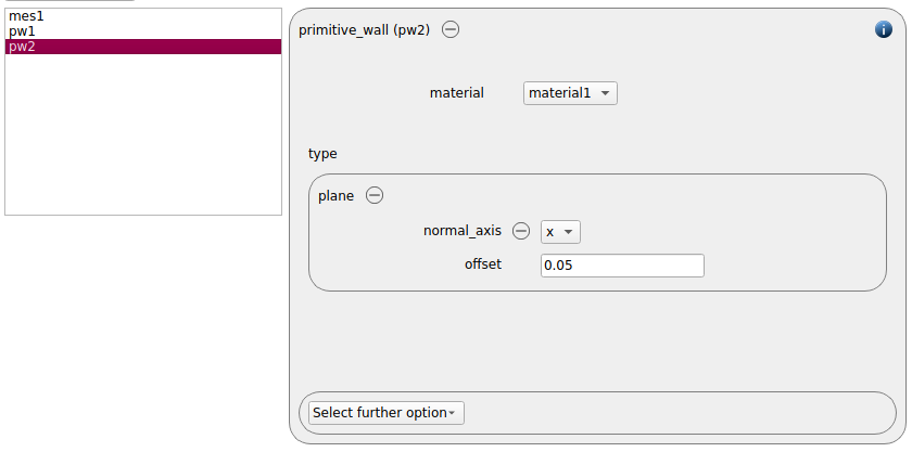
For obtaining a drum with solid walls, two primitive walls are used. Both of them are normal to the x axis, and they have an offset of -0.05 and 0.05 respectively:

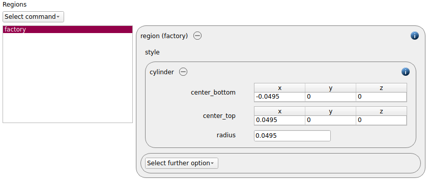
In the next step we generate a cylindric insertion region. The bottom center is set to (-0.0495, 0, 0) and the top center is set to (0.0495, 0, 0). The radius is set to 0.0495 meters.

Physics models

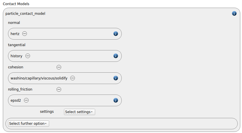
We use the standard contact model normal hertz and tangential history. As rolling friction model epsd2 is chosen. For simulating a liquid film at the particle surface, the formation of liquid bridges as well as their solidification we activate the cohesion model washino/capillary/viscous/solidify. Furthermore we set the limitLiquidContent setting to on.

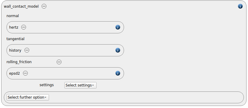
For the particle-wall contacts the wall contact model normal hertz, tangential history and rolling friction epsd2 is selected. There is no liquid transfer between particles and walls.

Next, the gravity is defined:

Per default the gravity has a magnitude of 9.807 and acts into negative z-direction. These defaults can be changed by either setting the magnitude or the direction manually; see enable_gravity command command.

We also activate the liquid transfer model:

Particles

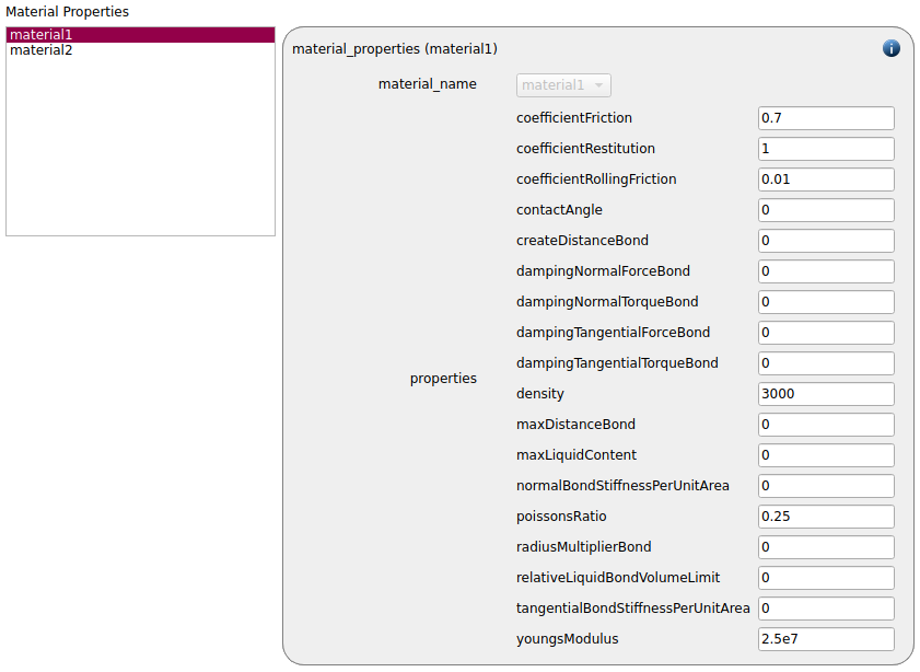
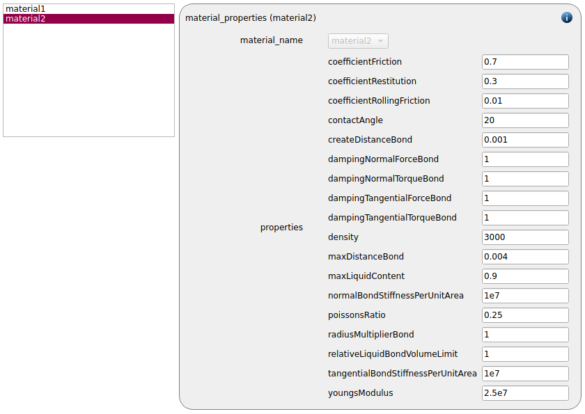
We set the material_properties command for the particle material:

	material1	material2
Density	3000	3000
Young’s modulus	2.5e7	2.5e7
Poisson ratio	0.25	0.25
Coefficient of restitution	1.0	0.3
Coefficient of friction	0.7	0.7
Contact angle	0	20
Max. liquid content	0.0	0.1
Coefficient of rolling friction	0.01	0.01
Create distance bond	0	0.001
Max. distance bond	0	0.004
Normal stiffness / unit area	0	1e7
Tangential stiffn. / unit area	0	1e7
Radius multiplier bond	0	1
Relat. liquid bond volume lim.	0	1
Damping normal force bond	0	1
Damping normal torque bond	0	1
Damping tangential force bond	0	1
Damping tangential torque bond	0	1

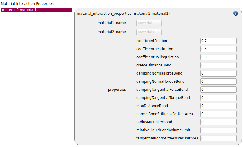
Since two different materials are used, we must also set the material interaction properties:

	material1 & material2
Coefficient of restitution	0.3
Coefficient of friction	0.7
Coefficient of rolling friction	0.01
Create distance bond	0
Max. distance bond	0
Normal stiffness / unit area	0
Tangential stiffn. / unit area	0
Radius multiplier bond	0
Relat. liquid bond volume lim.	0
Damping normal force bond	0
Damping normal torque bond	0
Damping tangential force bond	0
Damping tangential torque bond	0

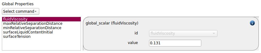
The selected physical models also require the definition of several global scalars:

	value
Fluid viscosity	0.131
Maximal relative separation distance	0.2
Minimal relative separation distance	0.05
Surface liquid content initial	1e-6
Surface tension	23e-3

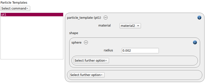
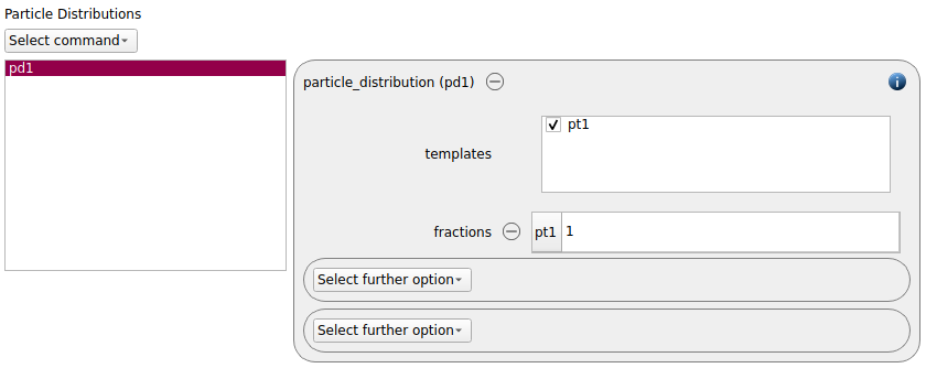
A spherical particle template with a radius of 0.002 is generated and used in a particle distribution:

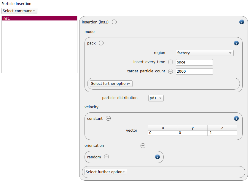
An insertion command command of type pack is created, which adds 2000 particles with a velocity of 1 m/s in negative z-direction. The orientation of the particles during insertion is set to random for avoiding undesired and unphysical alignment.

Simulation control

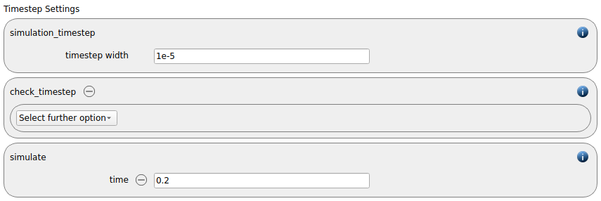
In the next section we define the simulation time step and the total simulation time.

For an optimal usage of the resources the load balancing is switched on:

Output settings

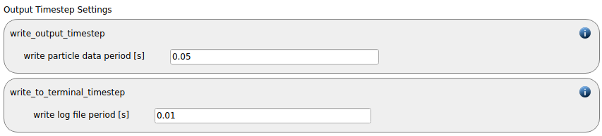
In this tab we first define the timestep width for the file and the terminal output:

The default output_settings command command is used:

Simulation and results

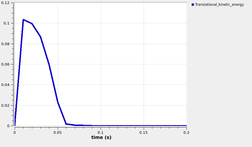
This was the last setting in for this calculation. Please save the project and change to the Simulation tab. After running the simulation the following curve for the kinetic energy shows:

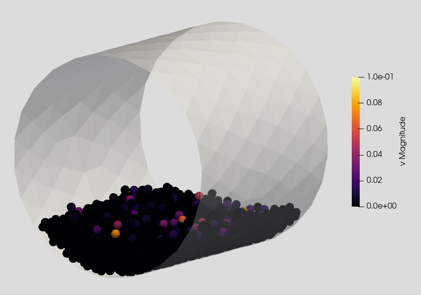
The result of this simulation is a settled particle bed that can be visualized with Paraview:

Simulation 2: Spray coating

We use the result of Simulation 1 as starting point for the spray coating simulation by deriving a simulation. The main changes in this case are the following: we add a rotational motion to the drum, the surface of the particle bed is detected and the spray is activated. Furthermore, we add a specific calculate command for visualizing both the cohesive and the solid bonds separately.

Meshes and regions

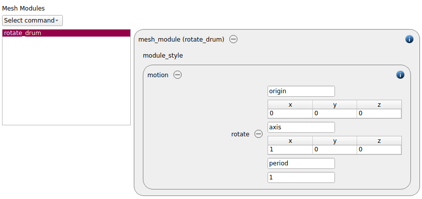
First, a mesh module of type motion is generated. The drum will rotate around the x-axis with a period of 1:

The mesh module must be added to the mesh in order to activate it:

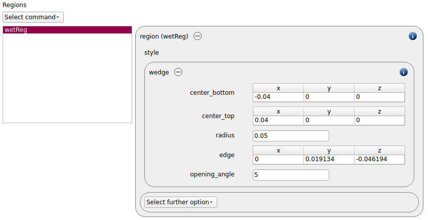
Instead of an insertion region we are now using a wetting region:

Particles

Since no further particles will be inserted, the insertion command, particle distribution and particle template can be removed (in that order).

Physics models

In the physics models tab we first add a command that detects particles that are at the surface of the particle bed:

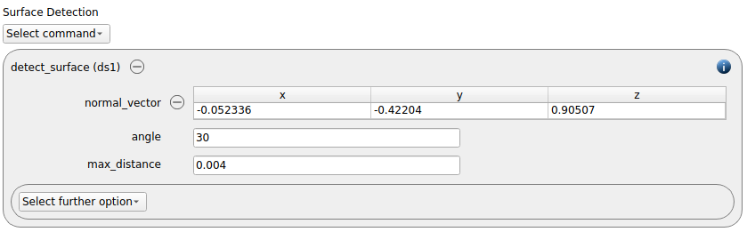
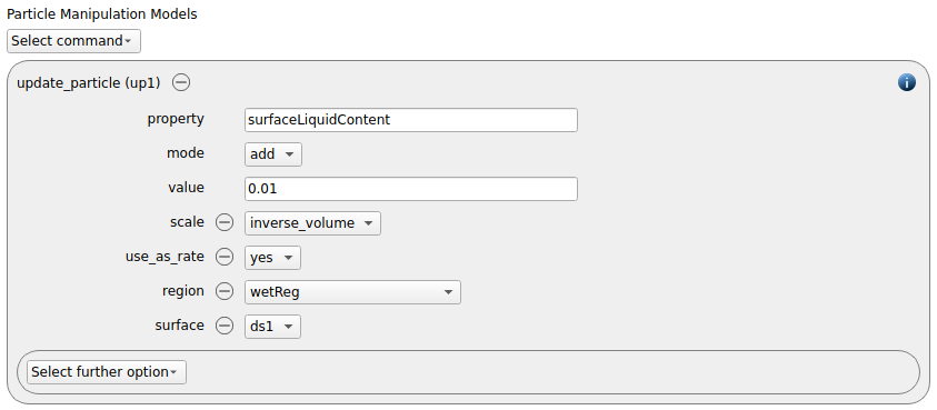
Then we use the update_particle command command to increase the surface liquid content of surface particles inside the specified wetting region:

Simulation control

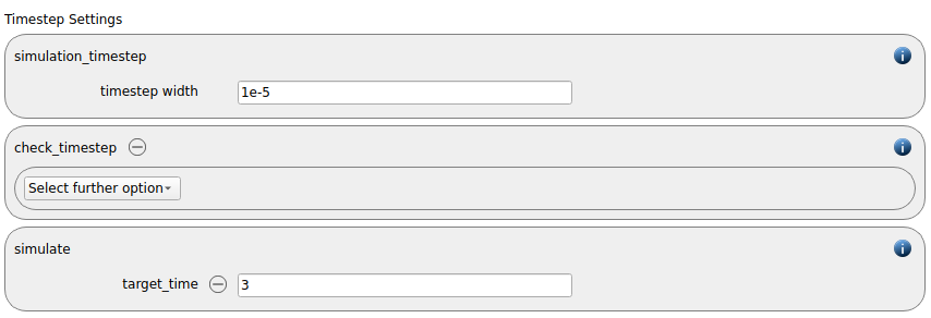
In the simulation control tab we change the run mode to a target time of 3 seconds.

Output settings

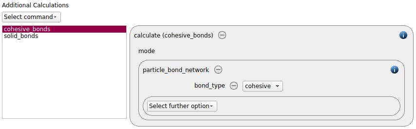
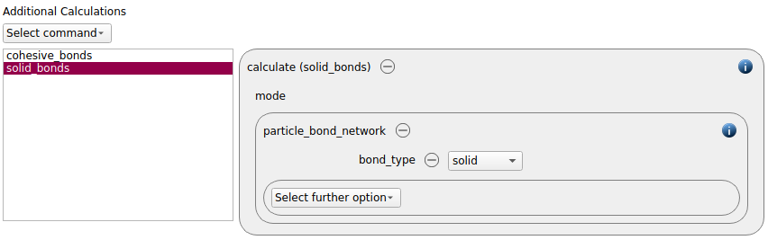
Two new calculate commands of type particle bond network are added to simplify the visualization of the cohesive and solid bonds as separate networks:

Simulation and results

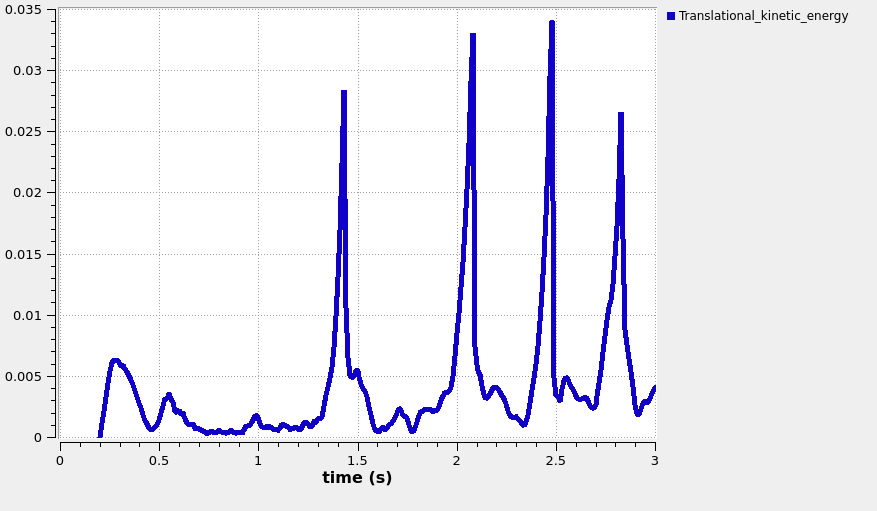
With this last setting the case setup is completed and the simulation can be launched. The graph below shows the kinetic energy of the particle bed:

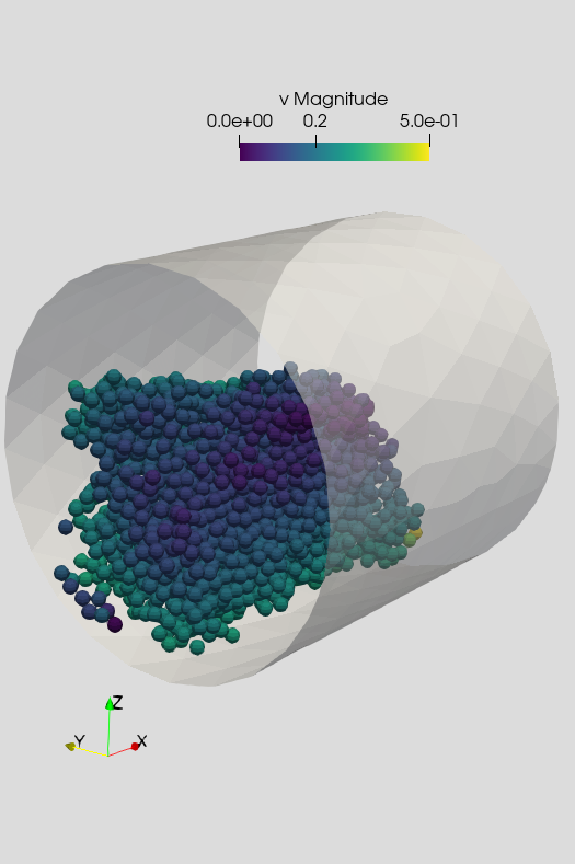
The results can also be visualized in Paraview, the image below shows the particles colored according to their velocity and the cohesive (light blue) and solid (pink) bond network:

Simulation 3 and 4: Reference simulation

For comparing the results with a run without solidification we duplicate the simulation tree. We unlock the Filling simulation by clicking on the small lock symbol

and replace the cohesion model to doc:washino/capillary/viscous <solver:gran_cohesion_washino_capillary_viscous>:

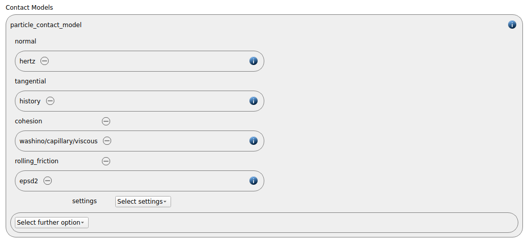
Please note that this step is also necessary for the derived spraying simulation!

The list of doc:material properties <solver:material_properties> and doc:material interaction properties <solver:material_interaction_properties> reduces significantly:

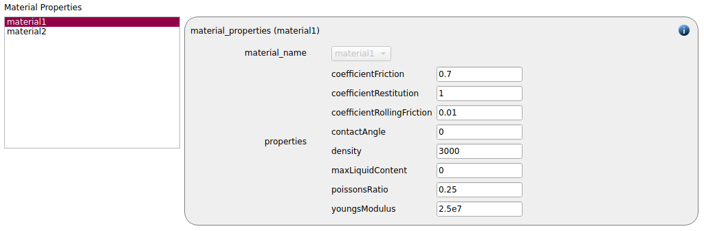
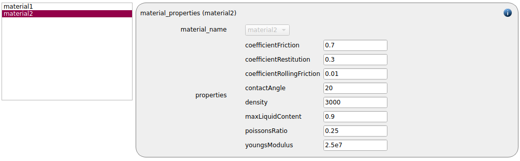
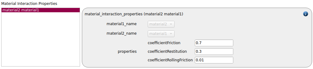
Finally, the additional calculate commands for the cohesive and solid bonds has to be removed from the Output settings section in the new spray simulation.

With this, the setup of the reference case is completed and the simulation can be launched.

When comparing the results in Paraview the difference becomes obvious: while the solidification case lease to the formation of a clump of particles, they remain separated in the pure liquid bridge case: