Heating up particles due to contact forces

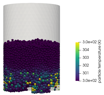
In this testcase we are inserting a mixture of spheres and superquadric particles in a cylinder with a rotor geometry at the bottom. Once the particles have settled the rotor starts to stirr the particles. The energy dissipated by the normal and tangential contact forces leads to an increase of the particle temperature. The image below shows the particle bed colored with respect to temperature:

The testcase consists of two separate Simulations, one for the filling and one for the stirring / heating part. While the heat conduction model has to be active from the beginning the surface heating model can be switched on when needed.

Name of the case: Project_Contact_Heating

Simulation 1: Generate the particle packing

General settings

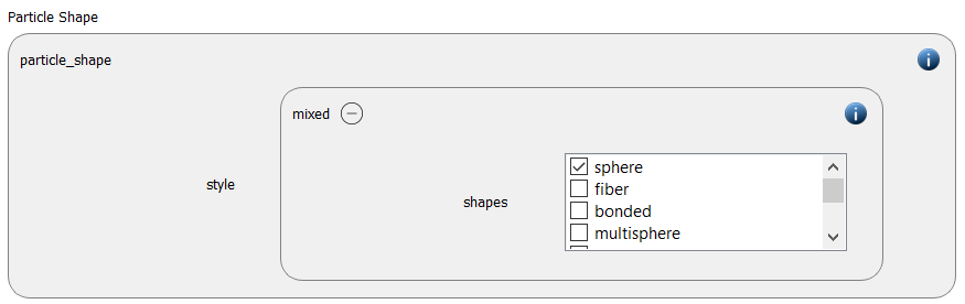
In this simulation we use spheres and superquadric particles and combine them with the particle_shape command mixed:

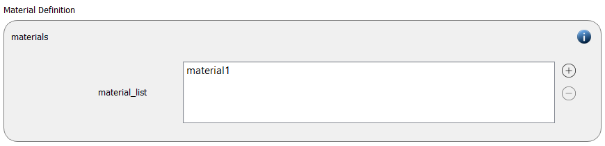
A material with name material1 is defined:

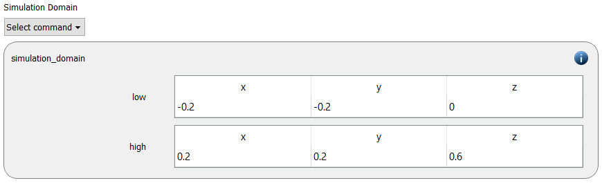
The simulation domain is defined with x and y dimensions ranging from -0.2 to 0.2 meters and z dimensions ranging from 0 to 0.6 meters:

Meshes and regions

The geometry consists of two meshes, a cylindric container and a rotor:

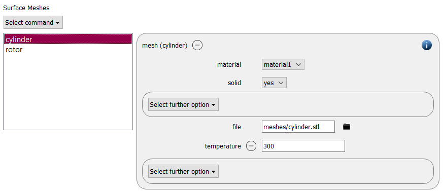
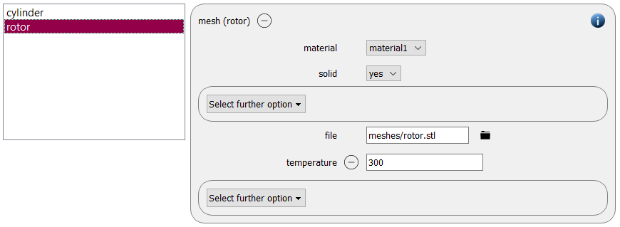
Both meshes have a temperature of 300 K, which remains constant throughout both simulations.

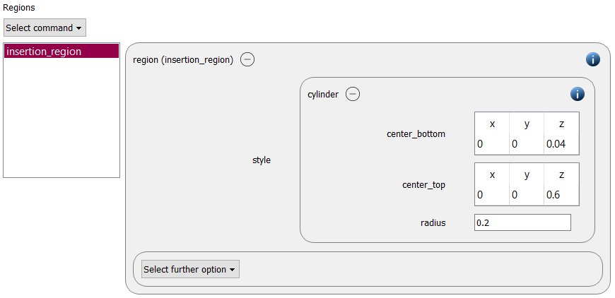
For the particle insertion later on we require an insertion region command:

Physics models

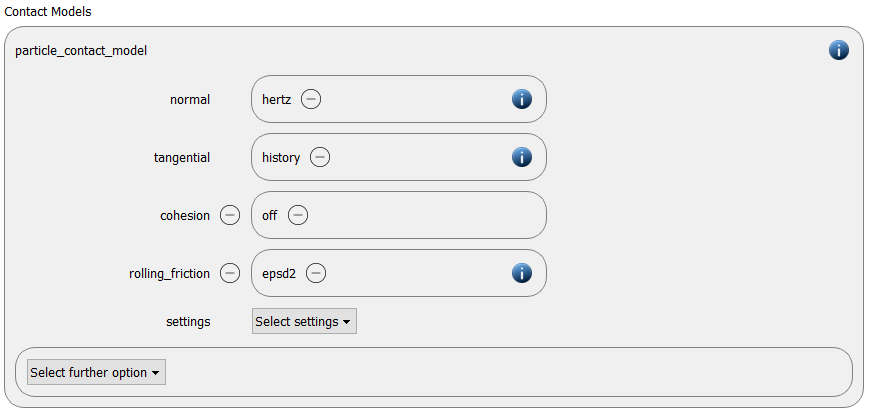
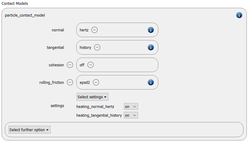
In the next step, the definition of the physics models takes place. For the particles we use the normal contact model hertz, the tangential model history and the rolling friction model epsd2.

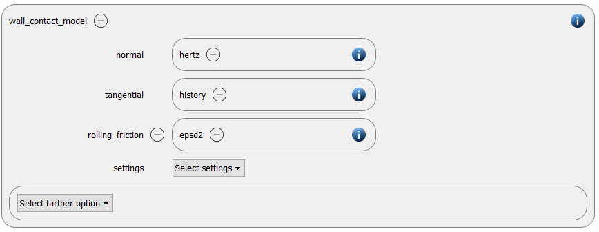
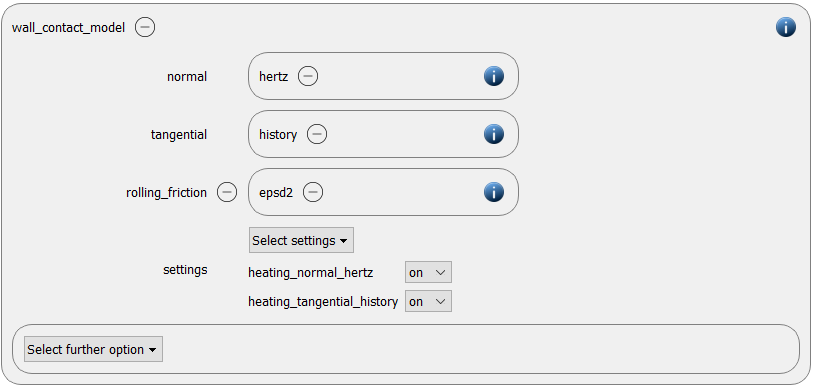
Since we added meshes in the previous section, also a wall contact model was added automatically in this section. We use the same contact models as for the particles:

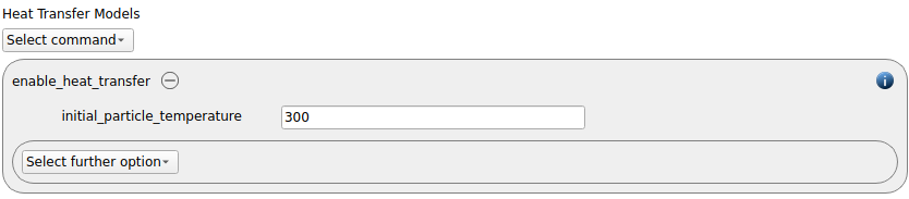
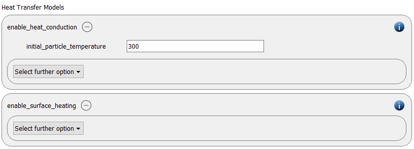
The heat transfer model is also activated in this section, just as the walls also the particles get an intial temperature of 300 K:

Finally also the gravity is defined:

Per default the gravity has a magnitude of 9.807 and acts into negative z-direction. These defaults can be changed by either setting the magnitude or the direction manually.

Particles

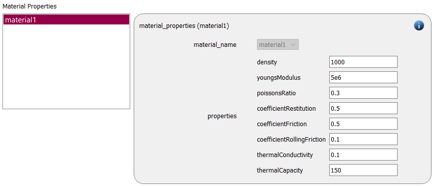
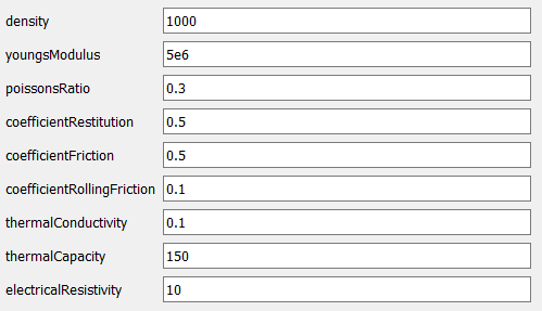
In the general settings tab we introduced one material. Here we define the required material properties.

	material1
Density	1000
Young’s modulus	5e6
Poisson ratio	0.3
Coefficient of restitution	0.5
Coefficient of friction	0.5
Coefficient of rolling friction	0.1
Thermal conductivity	0.1
Thermal capacity	150

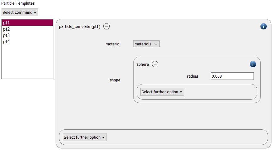
In the next step the particle templates are generated. First we define two sphere-templates, which only require the definition of the radius:

Template name	radius
pt1	0.008
pt2	0.01

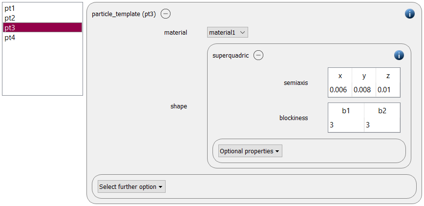
Then we add two superqudric particle templates:

Template name	semiaxis			blockiness
	x	y	z	b1	b2
pt3	0.006	0.008	0.01	3	3
pt4	0.005	0.01	0.015	3	3

Note

Multisphere and superquadric particles can be generated with the aid of the Multisphere and Superquadric Builder (Tools / Non-spherical particles). The multisphere templates can be saved as files and included in the respective template, the suerquadric templates are directly added to the simulation.

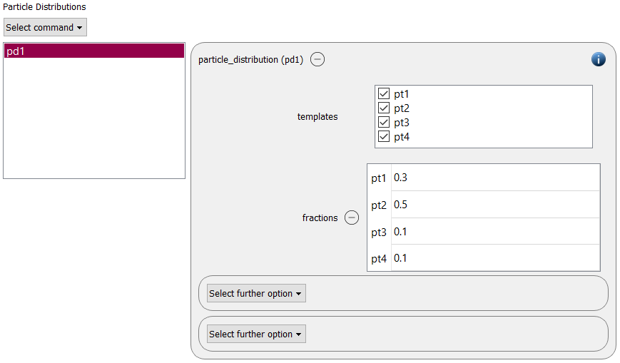
These four templates are used to define a particle distribution:

An insertion command command of type pack is used to insert particles into the previously defined insertion region:

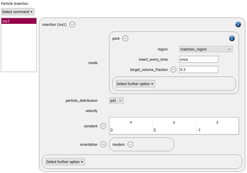
When non-spherical particles are used it is recommended to select “orientation random”, otherwise all templates are aligned at insertion.

Simulation control

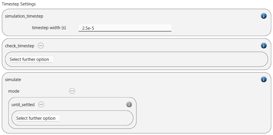
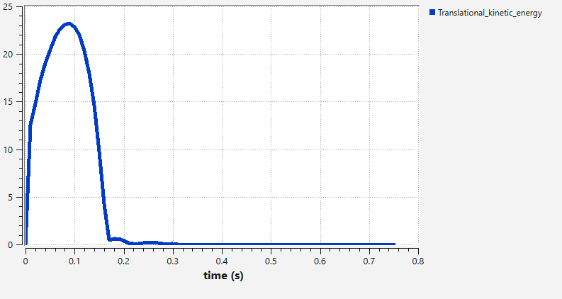
In this tab one first choses the time step settings such as the desired simulation timestep of 2.5e-5 seconds. Instead of selecting a pre-defined simulation time we use the simulate command in mode until_settled. The simulation will run until the kinetic energy in the domain falls below a threshold.

For an optimal distribution of the loads on the processors we activate the loadbalancing:

Output settings

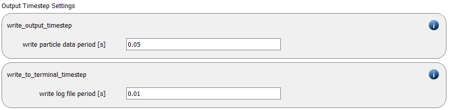
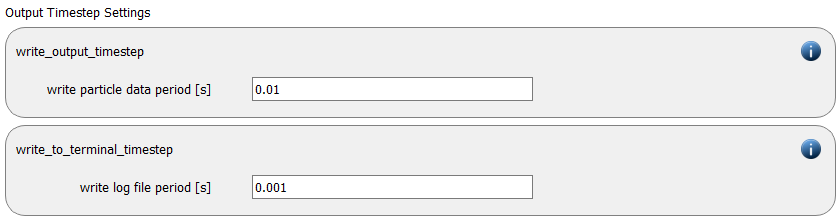
In this tab we first define the timestep width for the file and the terminal output:

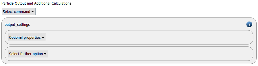
The output_settings command command takes care that all particle information and the meshes are written to files accordingly. Furthermore it triggers the output of global quantities such as the kinetic energy of the particles or total normal and shear stresses onto meshes in the terminal. Please note that if the output of per-cell information on meshes such as wear, velocity or stress are desired, the keyword mesh_properties has to be added and the required output has to be selected.

Running the simulation

After saving the case we can change to the Simulation section. By hitting the Start button we can start running the simulation either serially or in parallel, using mpi. Number of particles, kinetic energy as well as the forces on the geometry components can be visualized.

Result

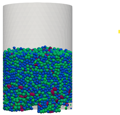
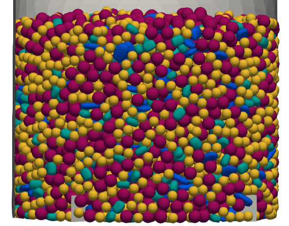
The result of the calculation can then be visualized with Paraview. The image shows the particles colored according to shapex (since it is easy to differ between the different particle templates then) after the settling is completed:

Simulation 2: Particle heating

This second simulation, which is derived from the filling case, will show the contact heating of the particles which are stirred by the rotor geometry. The main modifications of the case are the following:

• enable surface heating model (command + keyword in contact models)

• apply mesh motion to rotor and define deterministic simulation time

• measure average particle temperature in four regions

Meshes and regions

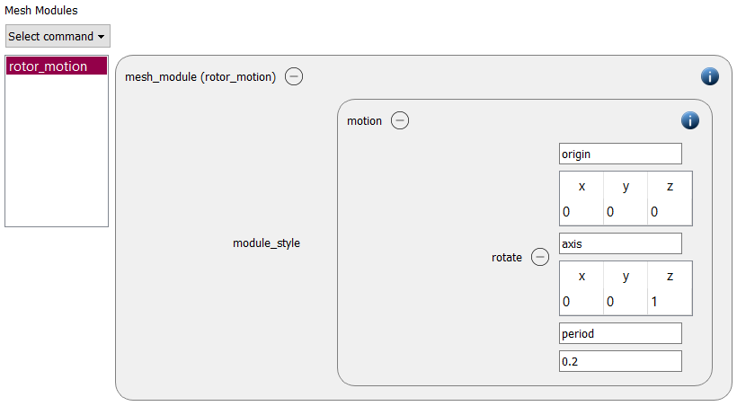
We start with generating a mesh module of type motion:

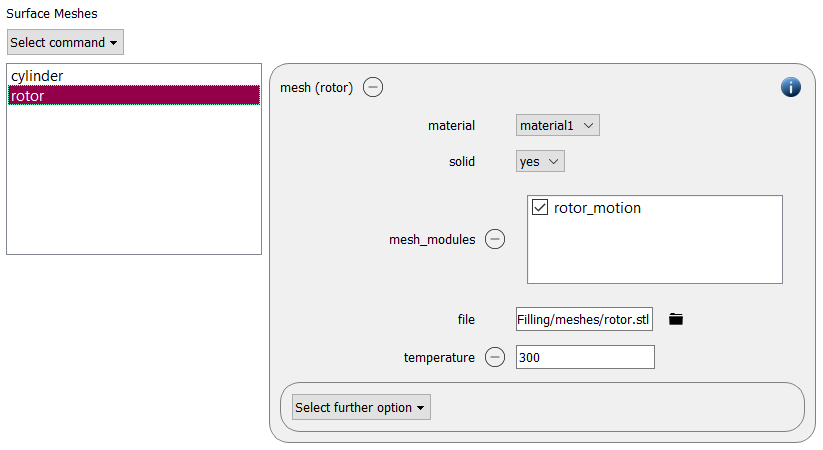
The mesh module is then activated for the rotor mesh:

The insertion region is no longer needed and we replace it by four cylindric regions for measuring the average particle temperature:

Region name	style	center bottom	center top	radius
r1	cylinder	(0,0,0)	(0,0,0.1)	0.2
r2	cylinder	(0,0,0.1)	(0,0,0.2)	0.2
r3	cylinder	(0,0,0.2)	(0,0,0.3)	0.2
r4	cylinder	(0,0,0.3)	(0,0,0.4)	0.2

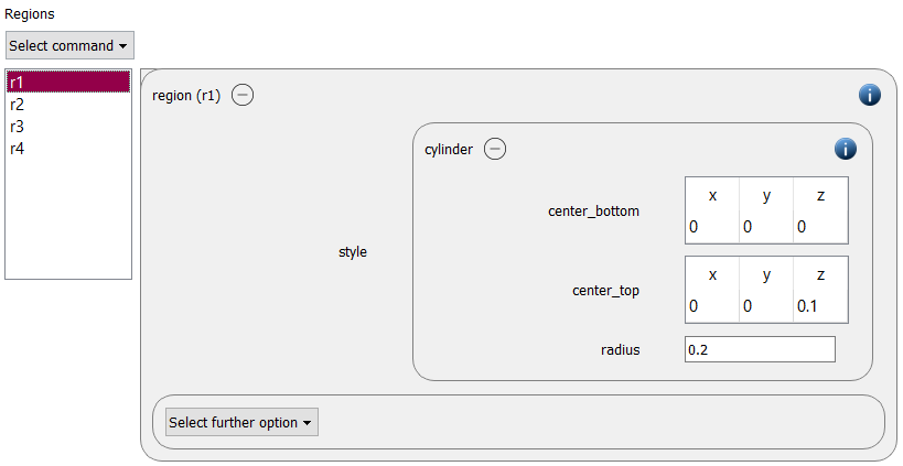
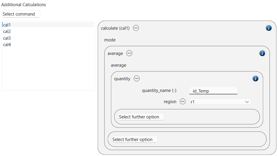
Please note that the reduce/region command we use later on requires the region names as input.

Physics models

For both the particle and the wall contact model we add the settings “heating_normal_hertz on” and “heating_tangential_history on”:

Then, in the “Heat Transfer Models” section we add the command enable_surface_heating command:

Particles

In the particles tab we must add a value for the electrical resistivity:

Next, we can delete the insertion command, the particle distribution and also all the particle templates (in this order):

Simulation control

In the simulate command we change to a deterministic simulation time of 0.5 seconds:

Output control

For capturing the motion of the rotor accordingly we decrease the output intervals:

For calculating the average temperature in the specified regions we add four calculate average commands. The particle temperature Temp can be accessed through the quantity id_Temp:

Running the simulation

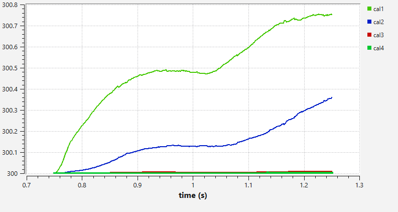
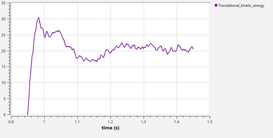
After launching the simulation (e.g., in parallel, on 2 cores) we can visualize both the temperature and the kinetic energy. It shows the heating of the particles with time, and the evaluation of the average particle temperature in the four regions shows the temperature distribution over the height.

Results

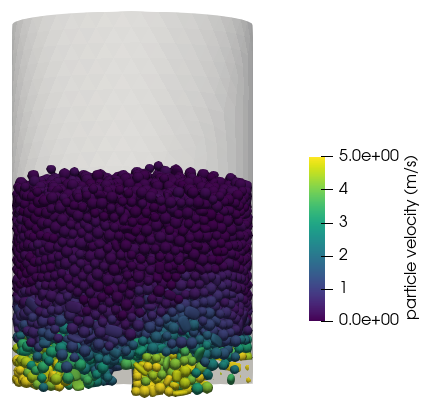
The results can be visualized in Paraview. The images below show the particle bed at the end of the simulation, colored by size, temperature and velocity.