Wear Modelling in a Ball Mill

This tutorial demonstrates the use of the Roessler–Katterfeld combined wear model, which evaluates total wear based on three mechanisms: impact cutting, impact deformation, and sliding. In the simulation, particles are first loaded into a baffled drum. Once they settle, the drum begins to rotate, and the wear generated by particle–wall interactions is computed.

Name of the case: Project_Wear_Ballmill

Insertion of particles

General settings

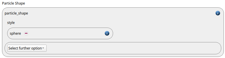
In this simulation we use particles of particle_shape type sphere:

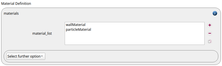
Two materials, ParticleMaterial and WallMaterial, are defined:

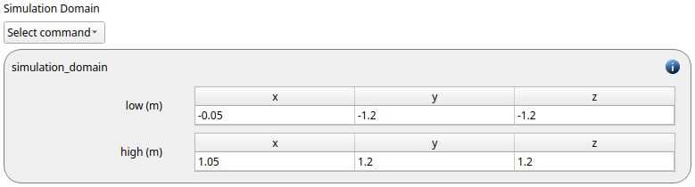
The simulation domain is defined with x dimensions ranging from -0.05 to 1.05 meters and the y and z dimension ranging from -1.2 to 1.2 meters:

Meshes and Regions

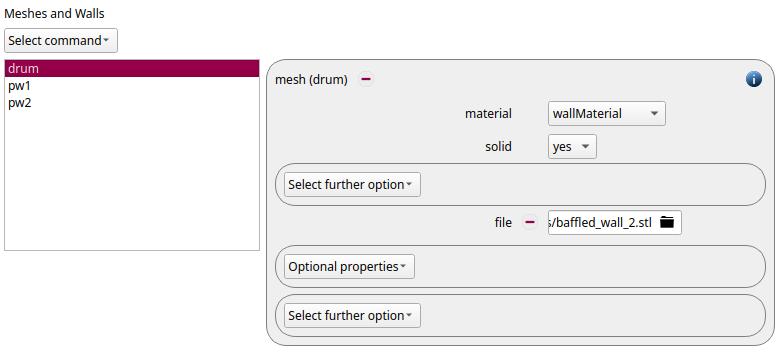
The setup uses a combination of meshes and primitive walls. All these components are of type WallMaterial.

We start with inserting the drum with baffles, using the mesh command:

Next we create the front and back walls using primitive walls of type plane

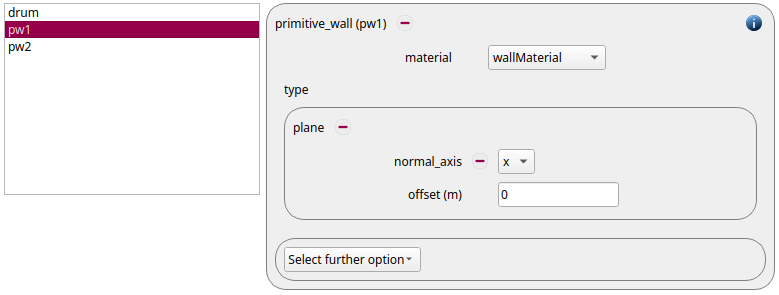
id	normal axis	offset
pw1	x	0
pw2	x	1

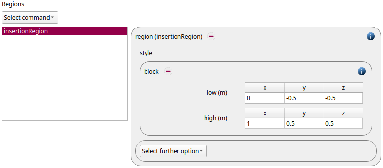
Finally we define the region that we will be using for the insertion:

Physics Models

In the next step, the definition of the physics models takes place. For the particles we use the normal contact model hertz and the tangential model history:

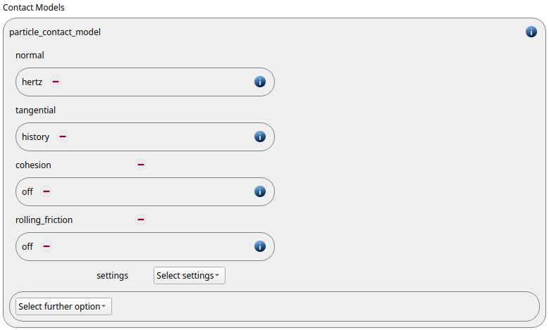
Since we added meshes and walls in the previous section a wall contact model was added automatically in this section. We use the same contact models as for the particles:

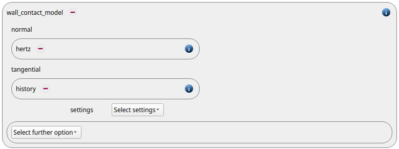
Finally also the gravity is defined:

Per default the gravity has a magnitude of 9.807 and acts into negative z-direction. These defaults can be changed by either setting the magnitude or the direction manually.

Particles

In the general settings tab we introduced two materials. Here we define the required material properties and material interaction properties.

	ParticleMaterial	WallMaterial
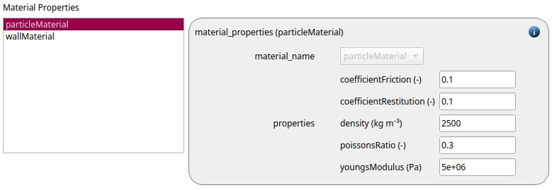
Density	2500	2500
Young’s modulus	5e6	5e6
Poisson ratio	0.3	0.3
Coefficient of restitution	0.1	0.1
Coefficient of friction	0.1	0.1

	ParticleMaterial / WallMaterial
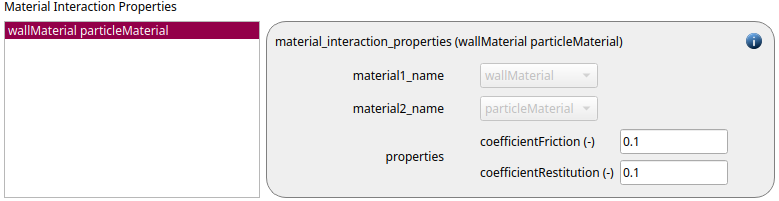
Coefficient of restitution	0.1
Coefficient of friction	0.1

We now define two particle templates , pt1 and pt2, both of which of shape sphere, both using ParticleMaterial with a radius of 3e-2 and 4e-2 meters respectively:

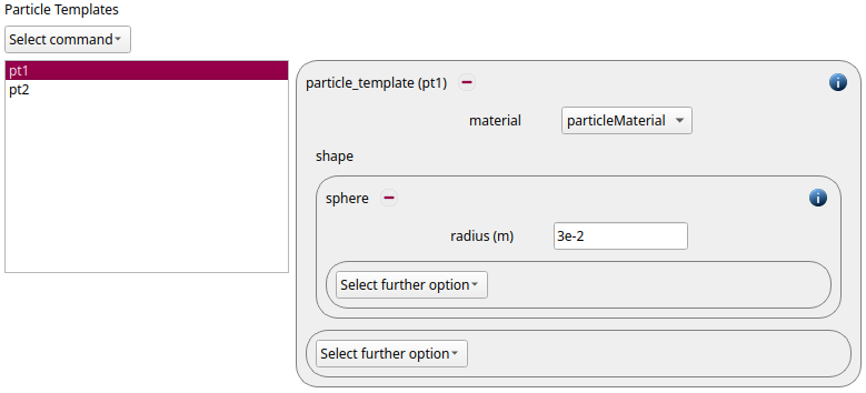
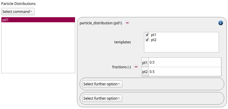
The two templates are used for a particle distribution:

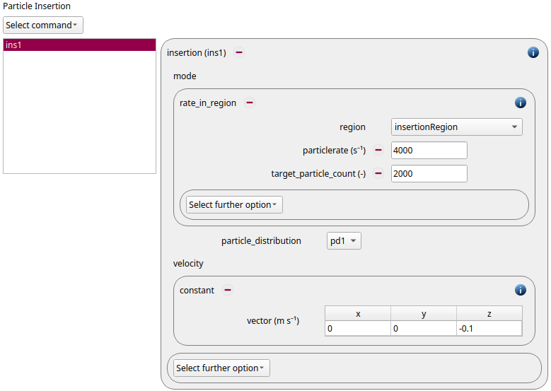
Finally we can define our insertion of mode rate_in_region:

	InsertionA
region	insertionRegion
particle_distriubtion	pd1
particlerate	4000
target_particle_count	2000
velocity vector	( 0, 0, -0.1)

Simulation Control

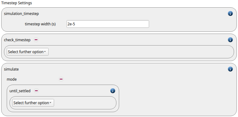
In this tab one first choses the time step settings such as the desired simulation timestep of 2e-5 seconds. Instead of defining a fixed simulation time, the simulate command is used with mode until_settled. Also the check_timestep command is enabled, which throws a warning when the time step exceeds 10 % of the Rayleigh or the Hertz timestep. These thresholds can be changed by setting an alternative value for hertz_fraction or rayleigh_fraction.

The enable_loadbalancing command is activated per default to ensure the optimal usage of the hardware resources.

Output Settings

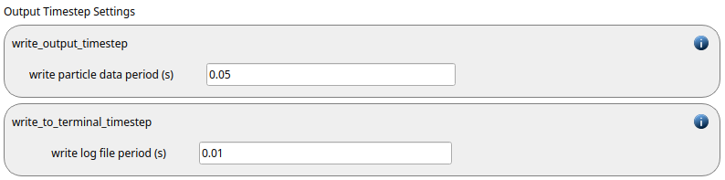
In this tab we first define the timestep width for the output to be 0.05 seconds and the terminal output to be 0.01 seconds:

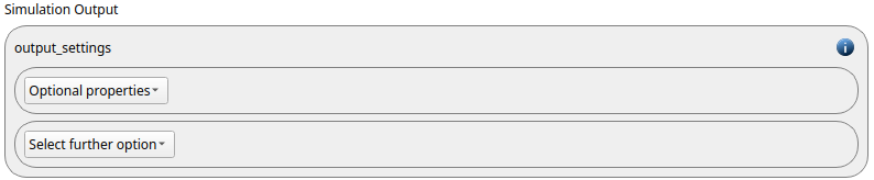
The output_settings command takes care that all particle information and the meshes are written to files accordingly. Furthermore it triggers the output of global quantities such as the kinetic energy of the particles or total normal and shear stresses onto meshes in the terminal. Please note that if the output of per-cell information on meshes such as wear, velocity or stress are desired, the keyword mesh_properties has to be added and the required output has to be selected.

Running the Simulation

After saving the case we can change to the Simulation section. Given the relativly low number of particles in this case using 2 processors for the MPI process is sufficient.

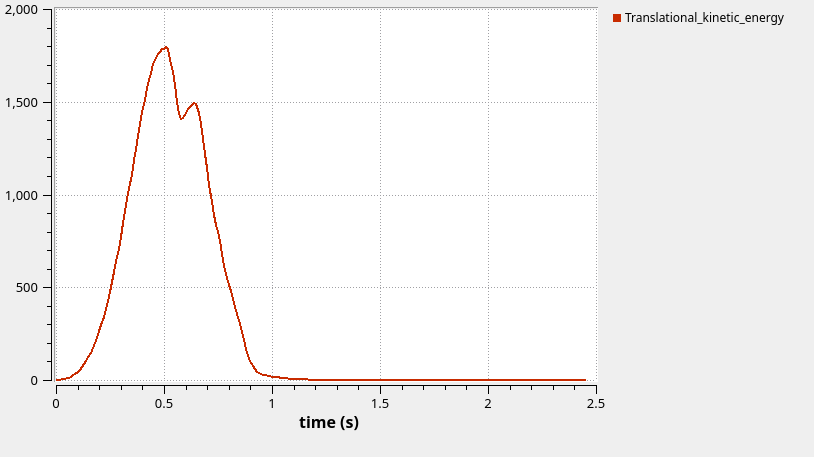
During the simulation run, different process quantities such as the kinetic energy can be visualized:

Postprocessing the results

After the simulation is completed, all data written with the output_settings command can be visualized automatically by going to the Visualization view and hitting the “Start Ovito” or “Start Paraview” button.

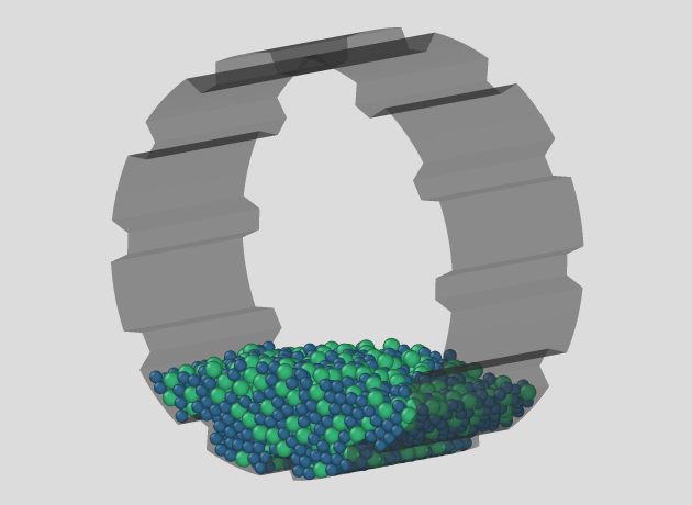
The image below shows the particle bed after setting is completed, the particles are colored according to the radius:

Rotation & wear

In this second simulation, both the motion of the drum and the wear calculation are added.

Meshes and regions

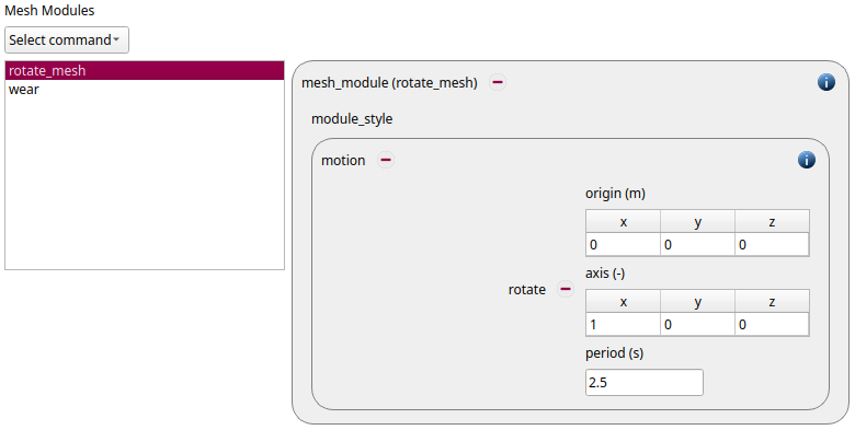
This is done by adding a new mesh_module of type motion with a rotation:

id	mesh_module	style	origin	axis	period
rotate_mesh	motion	rotate	( 0, 0, 0)	( 1, 0, 0 )	2.5

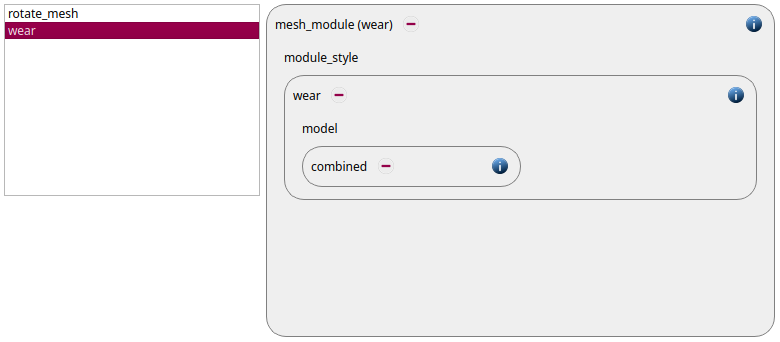
To activate the wear calculation, a mesh module of type wear is added, the combined wear model is selected:

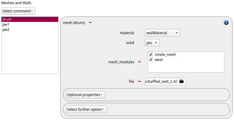
Finally, both models have to be actived for the drum mesh:

Particles

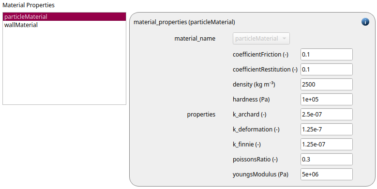
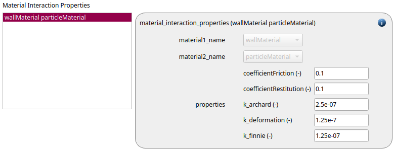
For the calculation of the wear models new material (interaction) properties (k_finnie, k_archard k_deformation and hardness) are required. We use 2.5e-07 k_archard, 1.25e-07 for k_finnie and k_deformation as well as 1e+05 for the hardness:

Next, the insertion command is removed:

Simulation control

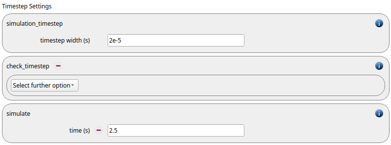
The simulation mode until_settled is replaced by a fixed simulation time of 2.5 seconds:

Output settings

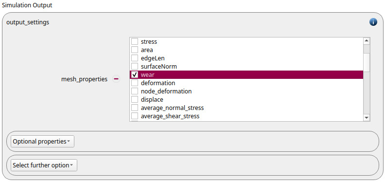
For being able to visualize the wear directly at the mesh, the mesh property wear is added in the output_settings command:

Running the simulation

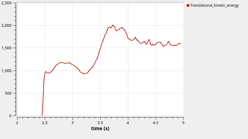
After launching the simulation (e.g., in parallel, on 2 cores) we can visualize both the kinetic energy and the wear:

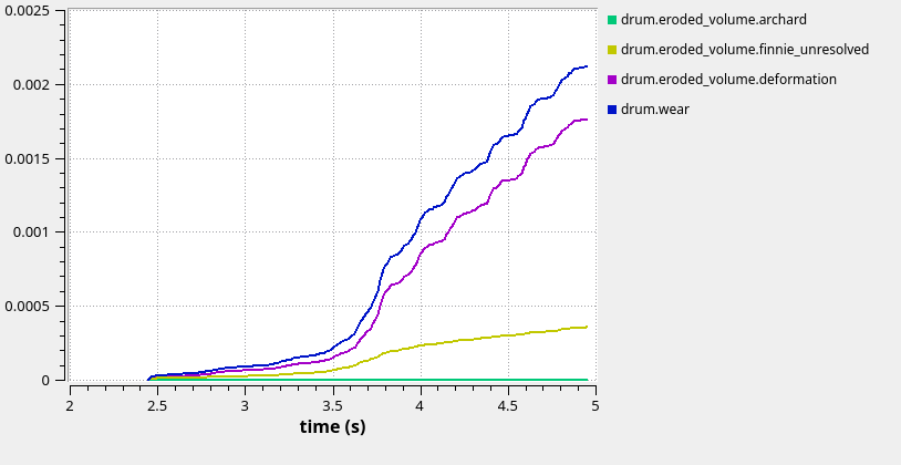
Postprocessing the results

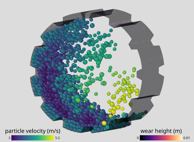
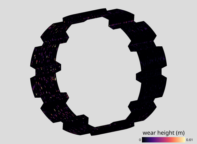
The results can be visualized in Ovito or Paraview. The images below show state of the simulation at the last time step, the particles are colored by velocity, the drum by wear height:

top