Particle Breakage

This tutorial consists of two simulations: in the first one a packing of spheres is generated, whereas in the second simulation the particles settle and the spheres break due to the forces that act onto the particles. It is crucial to use a mixed particle shape model for the simulations that allows both for fragments and spheres.

Simulation 1 - Creating a packing of spheres

We start with generating a new project and adding a simulation to it:

General settings

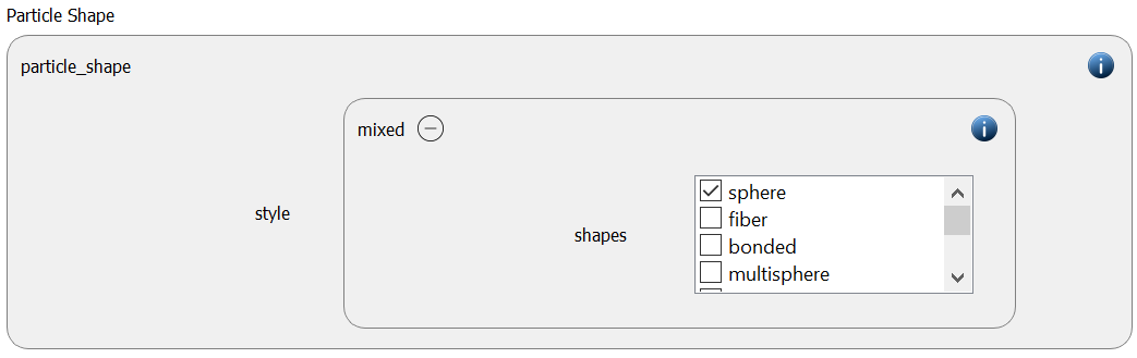
In this simulation we use particles of particle shape mixed and with the shapes sphere and fragments:

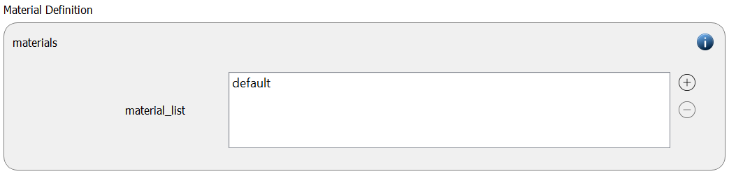
In this simulation only one material type is used (here called default):

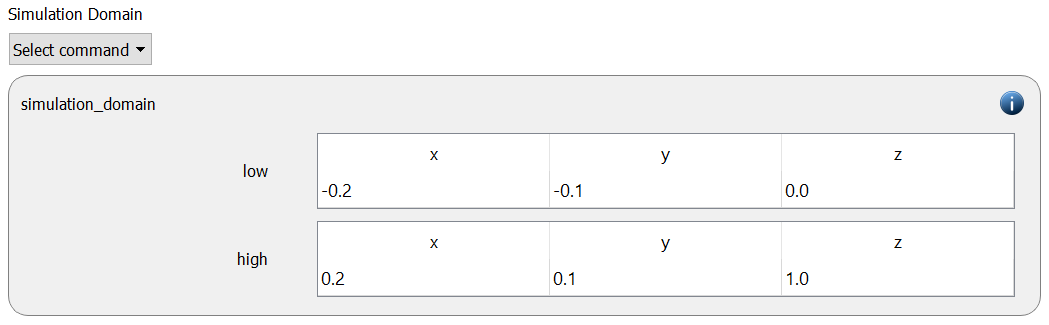
The simulation domain with x dimension ranging from -0.2 to 0.2, y dimension ranging from -0.1 to 0.1 and z dimension ranging from 0 to 1 is created:

Meshes and regions

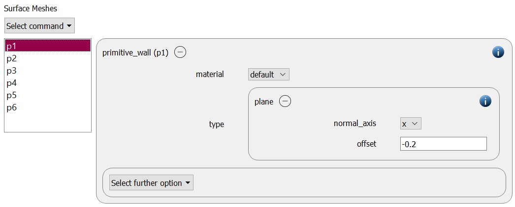
Six primitive walls of type plane are used to keep the particles inside the simulation domain (x: -0.2 and 0.2, y: -0.1 and 0.1, z: 0 and 1):

Physics models

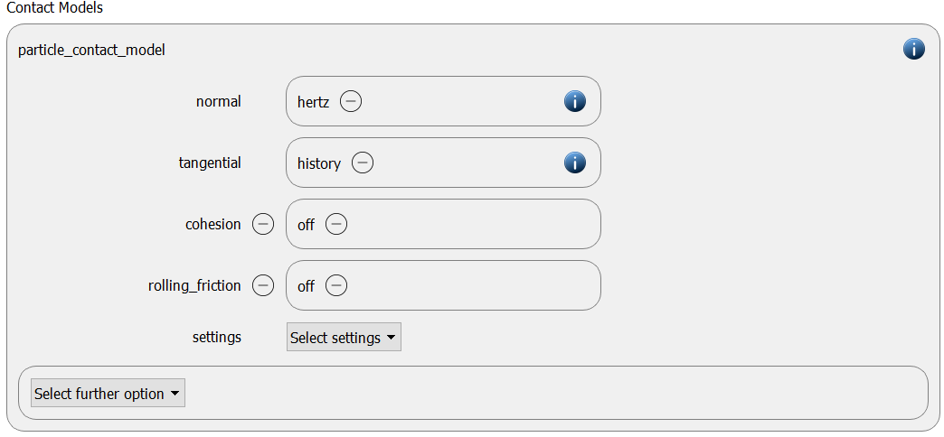
The contact models are now defined. For the particles we use the normal contact model hook and the tangential model history.

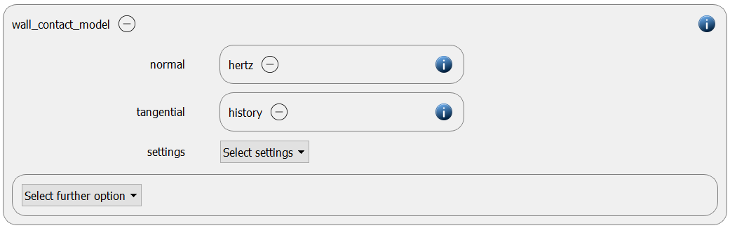
Since we primitive walls in the previous section, a wall contact model is also added automatically to this section. We use the normal contact hooke and the tangential model history:

The gravity is enabled by default:

Per default the gravity has a magnitude of 9.807 and acts into negative z-direction. These defaults can be changed by either setting the magnitude or the direction manually.

Particles

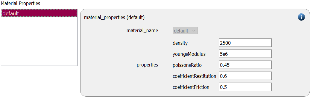
In the general settings tab we only defined a single material type (default), whose settings have to be specified here:

	default
Density	2500
Young’s modulus	5e6
Poisson’s ratio	0.45
Coefficient of restitution	0.6
Coefficient of friction	0.5

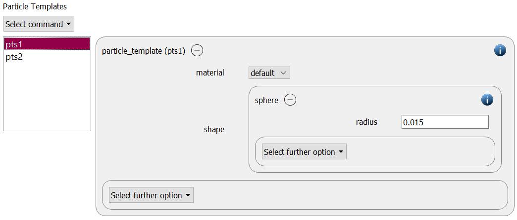
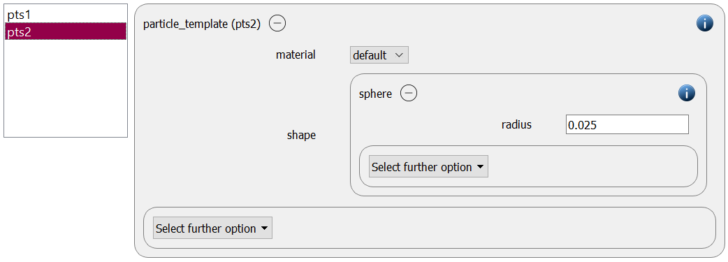
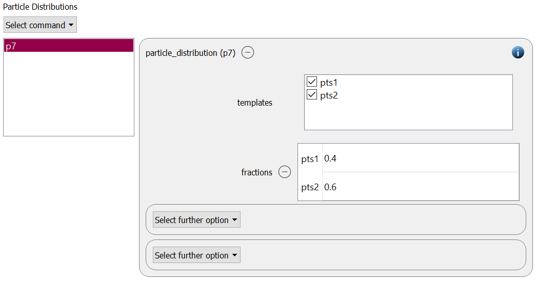
Two particle templates of type sphere with radii 0.015 and 0.025 are generated and used to form a particle distribution:

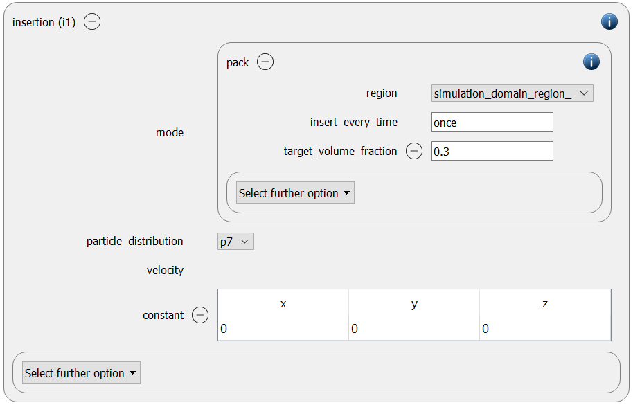
A pack of particles with a velocity of 0.0 m/s is inserted using an insertion command command with mode pack:

Simulation control

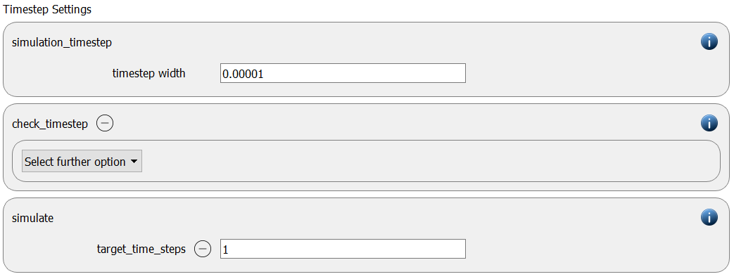
In this tab, we first define the time-step settings such as the desired simulation timestep of 1e-5 seconds and the total simulation time of a single time step. Per default also the check_timestep command command is enabled, which throws a warning when the time step exceeds 10 % of the Rayleigh or the Hertz time. These thresholds can be changed by setting an alternative value for hertz_fraction or rayleigh_fraction.

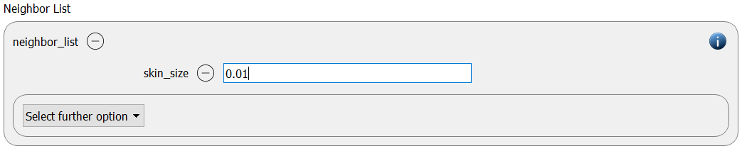
Another point that has to be taken care of is the correct setting of the skin size for building the neighbor lists:

Output settings

In this tab we first define the timestep width for the file and the terminal output:

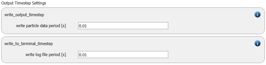
The output_settings command command the takes care that all particle information and the geometries are written to files accordingly. Furthermore it triggers the output of global quantities such as the amount or kinetic energy of the particles.

With this we have completed the setup of the first simulation. As soon as the project is saved one can change to the Simulation tab.

Running the simulation

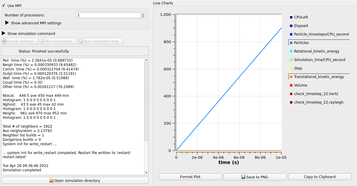
By clicking the run button the simulation is launched. Since only a single time step is conducted the simulation is completed almost immediately:

Simulation 2 - Settling and breakage

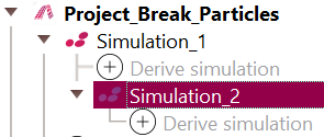
A new simulation is derived from the packing generation case:

Particles

We directly navigat to the Particle tab where we add a new particle template of type fragments:

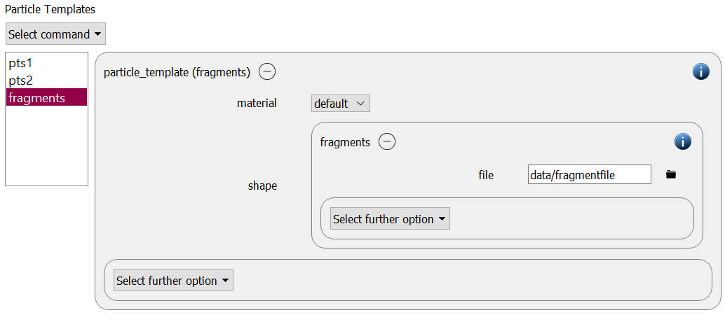
The fragments files contains the definition of the particle fragments that replaces the spherical particle when it breaks:

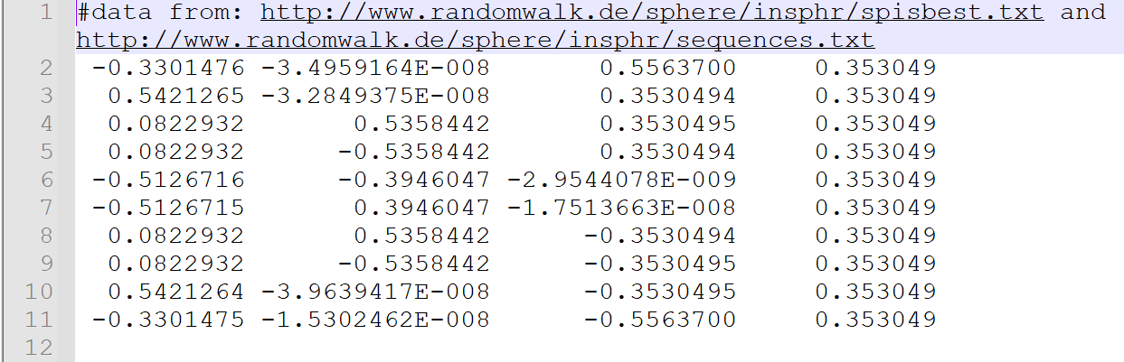
As soon as the project is saved, the fragments file is auto-saved to a data folder within the simulation directory.

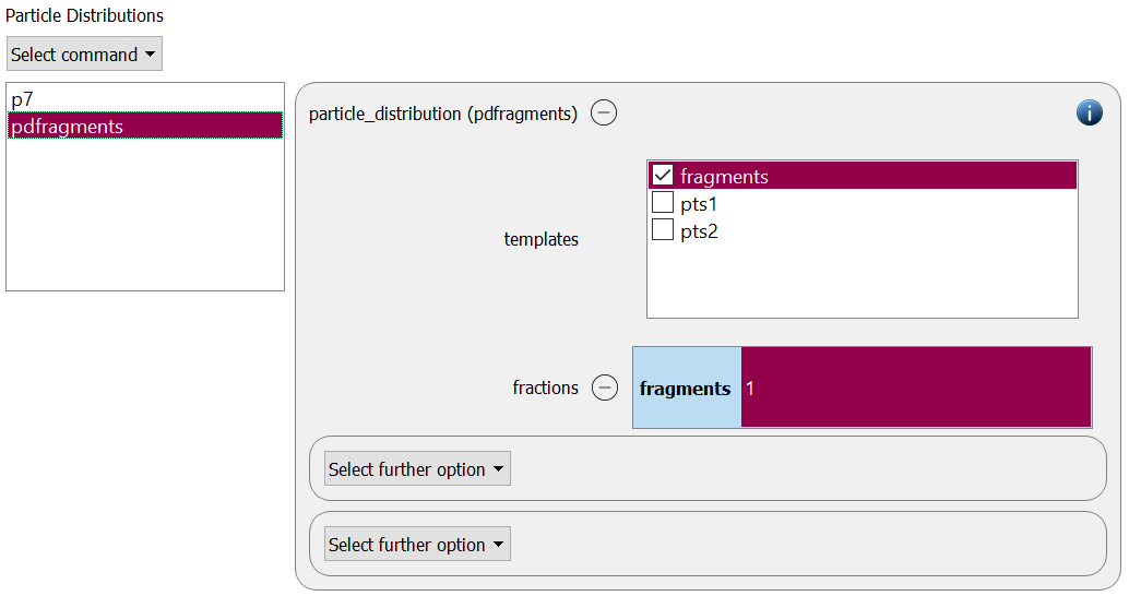
This particle template is now used to create a second particle distribution:

Physics models

We change to the Physics models tab and add a breakparticle/force command in the Particle Breakage section:

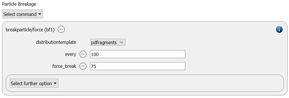
The force_break value is set to 75, checks for breakage should take place every 100 time steps.

Simulation control

The run time of this simulation is increased to one second:

This completes the setup of the settling and breakage simulation. After saving the setup we can move on to the Simulation tab.

Running the simulation

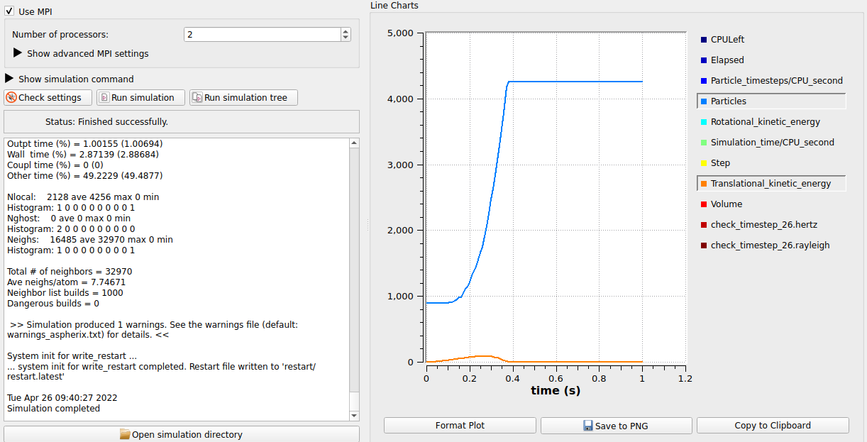
The simulation is launched by hitting the run button. One can see that the particles first start to settle under the influence of the gravity (increase of the kinetic energy). Once the particles start to collide they experience forces that cause the breakage of the spheres into fragments (increase of number of particles) until finally a settled case (constant number of particles, kinetic energy goes towards zero) is reached).

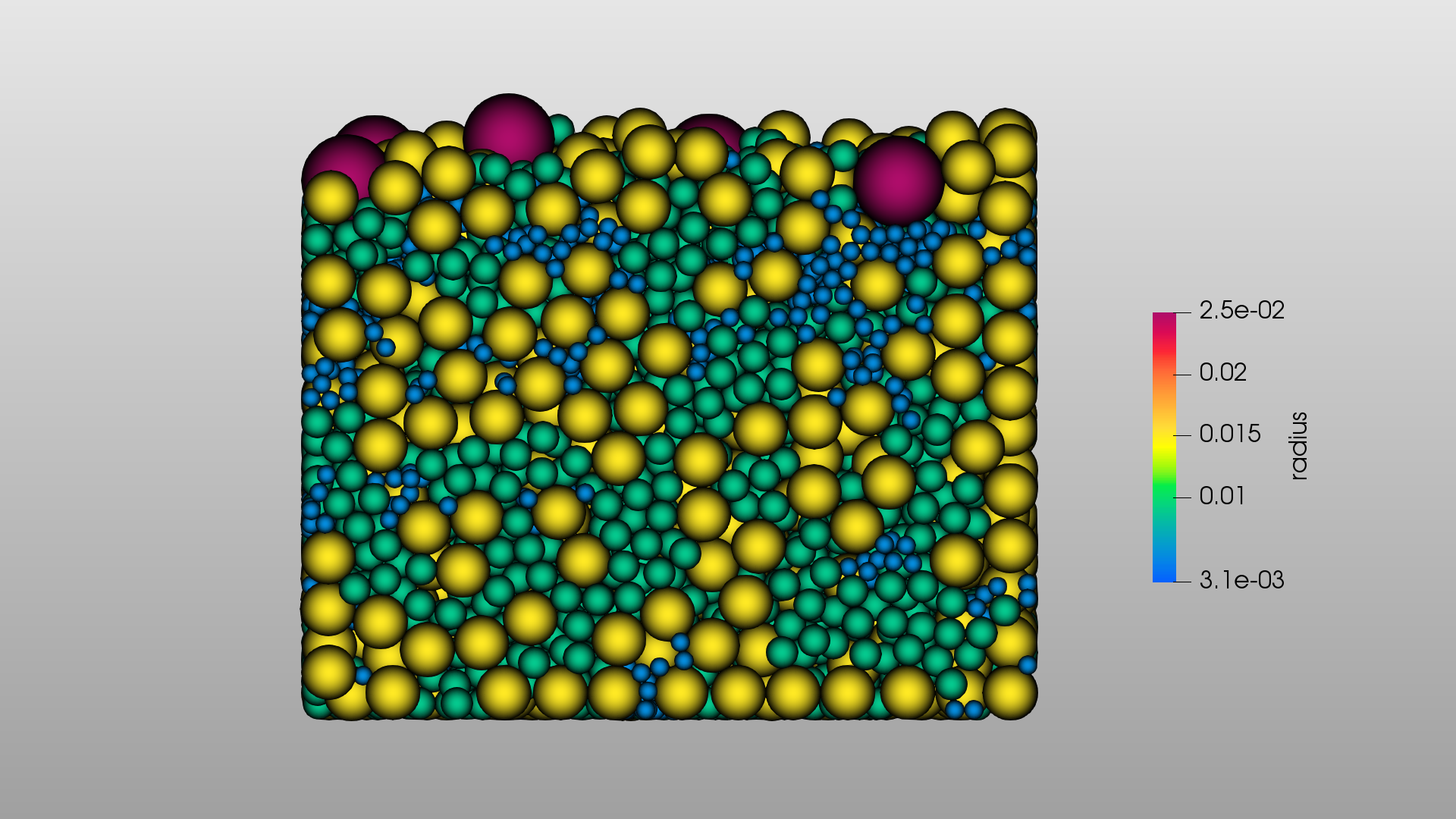
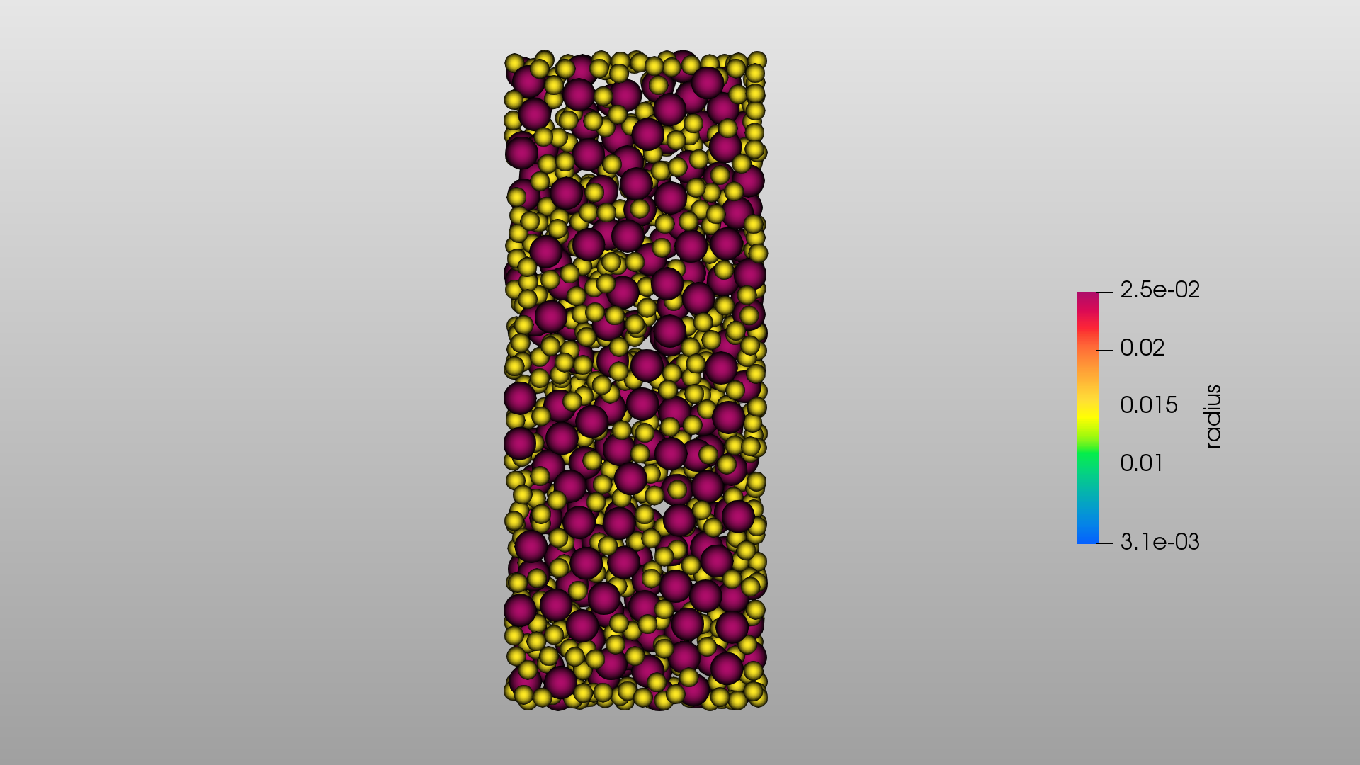
The images below show the initial and final state of the simulations.

Name of the case: Project_Break_Particles