 Home
HomeBubble Column
Warning
This tutorial is included in and relies on functionality that is available in the CFDEMcoupling-Premium package.
The simulations in this study are based on the experimental investigations of
three-phase hydrodynamics performed by Gan (2013). For his measurements,
Gan used a laboratory-scale cylindrical vessel of 0.152 m in diameter filled with a
salt-water mixture ( and
and
 at
at  )
up to a height of 1.05 m, as shown in Figure 1(a).
A sparger with a diameter of 0.03 m and a height of 0.05 m was placed in the center
of the column’s bottom. A continuous air stream, injected with a flow rate of
)
up to a height of 1.05 m, as shown in Figure 1(a).
A sparger with a diameter of 0.03 m and a height of 0.05 m was placed in the center
of the column’s bottom. A continuous air stream, injected with a flow rate of
 , was segmented by the sparger into
discrete bubbles with diameters between 0.7 mm and 2.3 mm.
In the experiment Phase Doppler anemometry (PDA) measurement at various heights of the
bubble column showed insignificant changes of the bubble size distributions (BSD).
Additionally, a third phase of solid particles was present: 20,000 monosized
acrylic beads of neutral density (
, was segmented by the sparger into
discrete bubbles with diameters between 0.7 mm and 2.3 mm.
In the experiment Phase Doppler anemometry (PDA) measurement at various heights of the
bubble column showed insignificant changes of the bubble size distributions (BSD).
Additionally, a third phase of solid particles was present: 20,000 monosized
acrylic beads of neutral density ( )
and a diameter of 3 mm were added, giving a total volume fraction
of
)
and a diameter of 3 mm were added, giving a total volume fraction
of  .
.
In the present simulations the geometry of Gan’s experiment case is discretized
using an appropriate computational grid, with the center part of the bubble column
having a cuboid shape that is composed of  cubic cells
with a constant edge length of 0.01 m, as shown in Fig. 1(b). In order to represent
the sparger, the inner
cubic cells
with a constant edge length of 0.01 m, as shown in Fig. 1(b). In order to represent
the sparger, the inner  cells at the bottom of the above
mentioned cuboid are left blank (they were not considered to be part of the
computational domain).
The water surface is modeled as a non-deformable interface using a slip condition for
the velocity at the outlet.
In contrast to the BSD of the experiment, bubbles with a constant diameter of
3 mm are injected right above the sparger with a velocity of
cells at the bottom of the above
mentioned cuboid are left blank (they were not considered to be part of the
computational domain).
The water surface is modeled as a non-deformable interface using a slip condition for
the velocity at the outlet.
In contrast to the BSD of the experiment, bubbles with a constant diameter of
3 mm are injected right above the sparger with a velocity of
 .
.
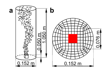
Figure 1: Schematic view of (a) the dimensions of the cylindrical bubble column,
(b) the cross sectional profile of the grid whereby the red square marks the sparger,
and (c) the bubble size distribution above the sparger
( ,
,  ).
).
Please note, that the solid particles are neglected in this case setup. Similar simulations with different contact models were conducted in Gruber (2015), where the impact of the solid particles was also assessed.
Note
This case is located in CFDEMcoupling/validationCases/bubbleColumn_Gan2013.
Models used
LES turbulence model
The drag model is enhanced with a stochasticDispersion forceSubModel which accounts for effects of turbulence acting on the particles. This model is configured separately in
constant/dispersionModel.dict.
A variant of this case with bubble breakup and coalescence is available activating breakup and coalescence models on the DEM side.
Note
The default setup of this case runs for a shorter time and acquires statistics for
a very short time. To recreate the results shown in this article comment the
settings changes in prerun_TH.sh.
Results
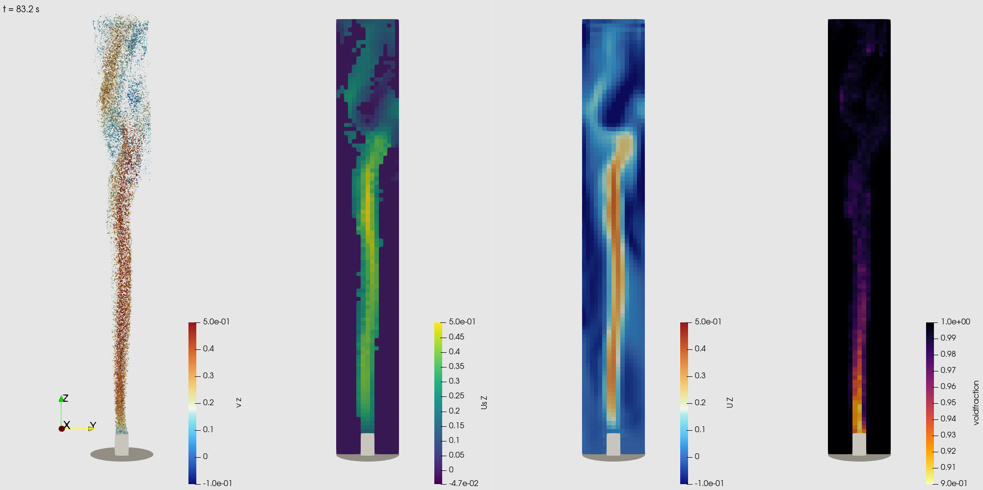
Figure 2: Snapshot of the base variant with constant bubble size. A video in real-time is available here .
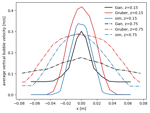
Figure 3: Statistical results of the base variant with constant bubble size.
The average bubble velocity was computed for  .
.
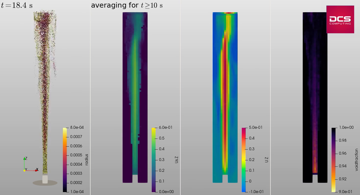
Figure 4: Snapshot of the variant with bubble breakup and coalescence. Watch the real-time video .
References
[1] Z.W. Gan, Hold-up and velocity profiles of monosized spherical solids in a three-phase bubble column, Chem. Eng. Sci. 94, 291–301, 2013
[2] M. Gruber, Hydrodynamics, Mass Transfer and Chemical Reactions in Bubble Columns, PhD Thesis, Graz University of Technology, 2015