Thermal Chute Wear

In the presented case particles are inserted into a domain via an insertion face. They drop onto a slowly rotating chute on which the wear stress is calculated. The particles slide down the chute and fall into a cold box with a temperature of 100 K, while the chute and the particles have an initial temperature of 300 K (cf. image below).

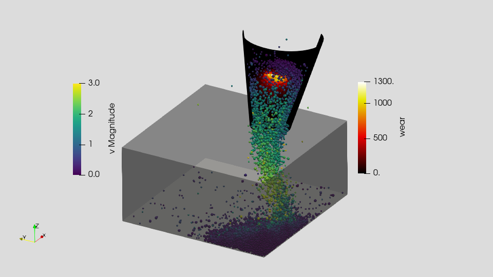
The image shows the particle temperature and the wear on the chute. The particles cool down as soon as they reach the bottom of the box.

Name of the case: Project_Thermal_Chute_Wear

Setting up the simulation

When Aspherix® GUI is launched, the user can chose between loading a recent or generally an existing project, opening a tutorial case or creating a new project. We start with the latter. The project name is Project_Thermal_Chute_Wear and also a flie path to which the tutorial will be saved has to be selected:

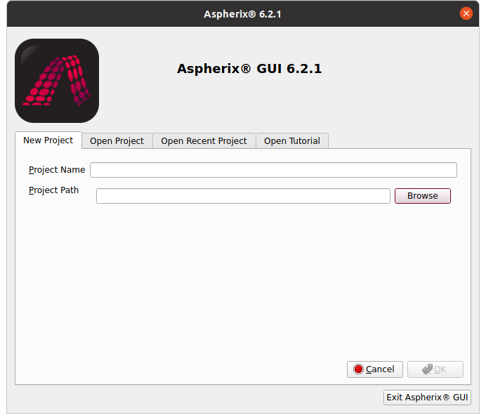
It is possible to change project names at a later point in the Projects View.

General settings

In the General Settings tab particle shape, the materials and also the simulation domain are defined. The boundary_conditions command command in the Simulation Domain section can be used to change the boundary type from fixed to periodic boundaries. Please note that none of these settings can be changed in derived simulations. It is neither possible to modify the particle shape type or to add futher materials in a dependent simulation. If you plan to use more materials at a later state, please add them from the beginning.

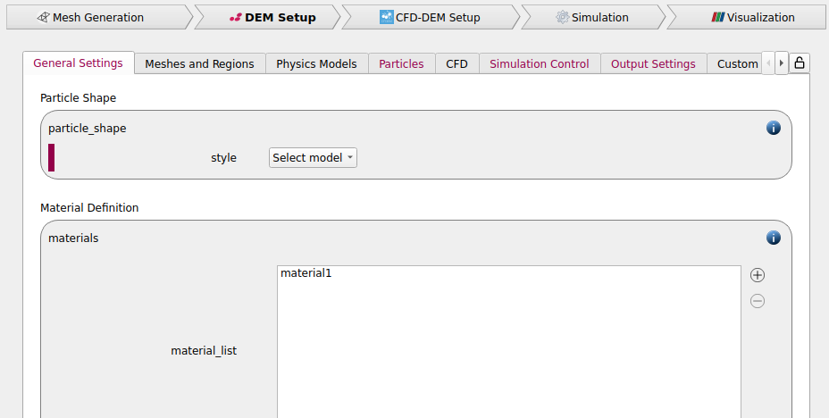
We start with setting the particle_shape command type to sphere:

Next, we define 3 materials command called particle1, particle2 and wallMaterial:

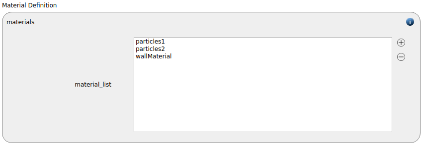
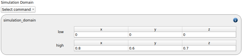
The simulation_domain command with x dimensions ranging from 0 to 0.8 m, y dimensions ranging from 0 to 0.6 m and z dimensions ranging from 0 to 0.7 m is created:

Warning

Per default, meshes have to be fully contained in the simulation domain at all times. This restriction can be lifted by setting the mesh option remove_protruding_mesh_elements to yes - all mesh elements that are (fully or partially) out

Meshes and regions

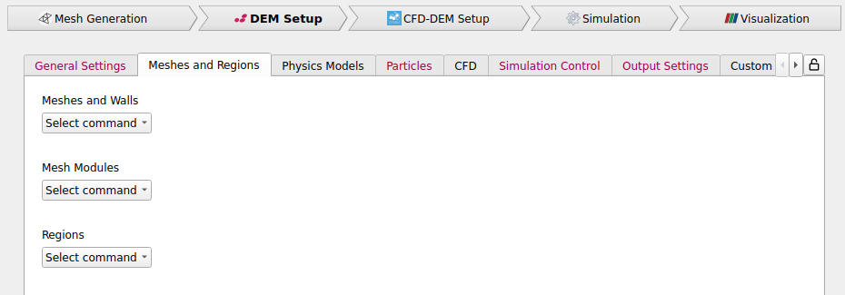
Aspherix® provides the possibility to use mesh command files (surface mesh files, stl-format) or primitive elements (planes, cylinders) as walls. Furthermore meshes can also be used for insertion of massflow measurements, in these cases the solid option must be set to no and the is_planar option must be set to yes. Advanced models for meshes such as motion (predefined, force-controlled, 6dof), wear, deformation, etc. are available in the form of mesh_modules. Mesh modules are defined through their commands and can then be applied to the respective mesh.

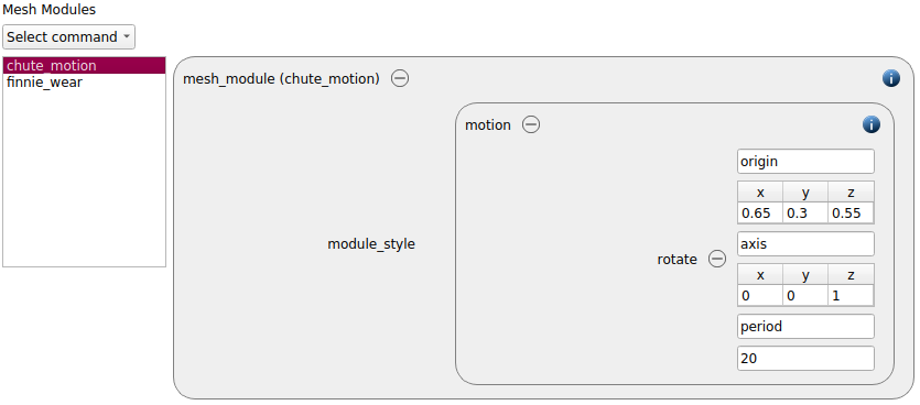
We first create a mesh module that defines the rotational motion of the chute:

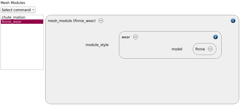
Then we add a second module for the calculation of the wear.

Remark: Please note that not all mesh modules can be combined with each other. At the same time there are mesh modules that require the application of other mesh modules beforehand. For more information concerning that topic please have a look at the documentation of the mesh modules.

We proceed with loading a mesh for the box in which the particles will fall:

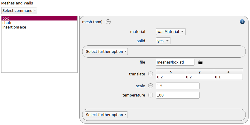
It is of material wallMaterial and has a temperature of 100 K. In contrast to this the chute has a temperature of 300 K:

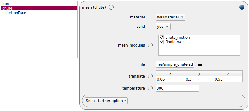
Both the motion and the wear mesh module are added to the chute. The creation of the wear mesh module automatically triggered the addition of a wear parameter to the material properties in the particles section.

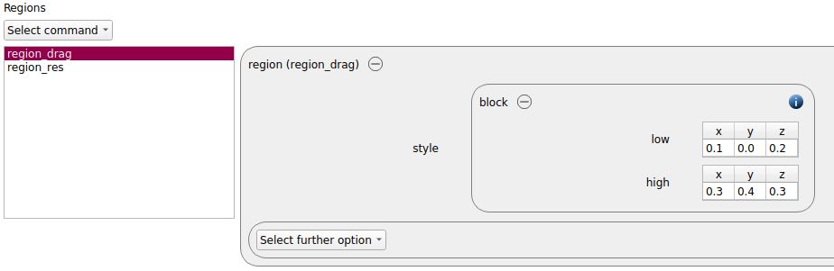
The user can define different kinds of regions, which can for example be used as insertion domains, for monitoring the particles’ residence time in particular areas or for imposing fluid-velocity fields. Available shapes are for example boxes, cones, cylinders, prisms / parallelepipeds and spheres. In the presented case a box is defined, in which drag force due to an external force (i.e. a fluid velocity field) will be imposed later on:

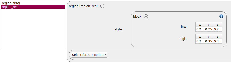
A second box is defined underneath the chute, it will be used for measuring the residence time:

Physics models

In this section we define the contact models as well as other physical models. As soon as walls are present in a simulation, the command for the wall contact model is added automatically. Other options include switching on heat transfer, adding forces such as a buoyancy or simply setting fixed velocities to groups of particles. Models for particle growth, breakage, liquid transport, evaporation, porous or spongy particles are available as well.

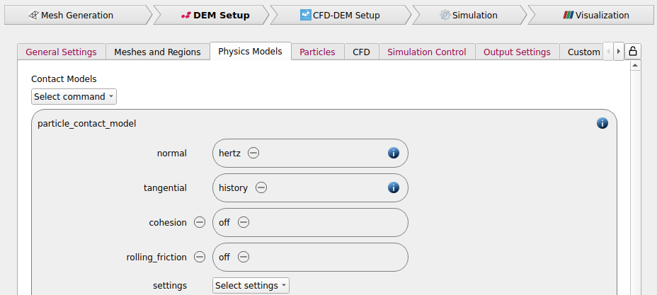
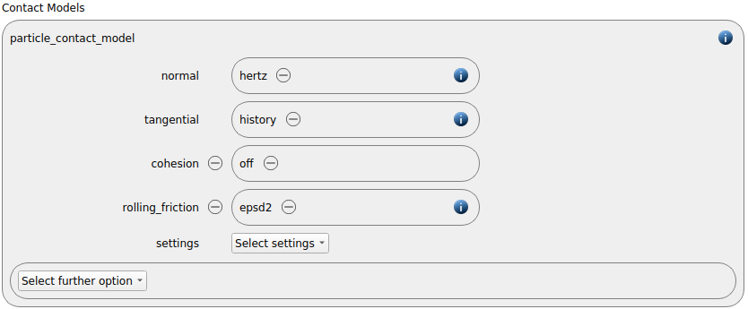
We start with the definition of the particle-particle contact model. We use the normal contact model hertz and the tangential model history. Furthermore the rolling friction model epsd2 is active:

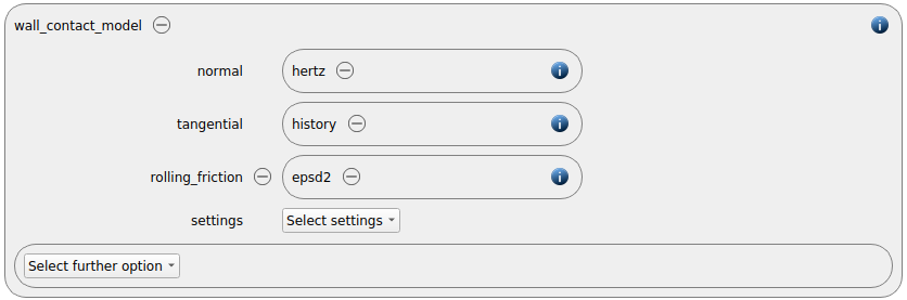
Since we added two meshes in the previous section also a wall contact model was added automatically in this section. We use the same properties as for the particle contact model:

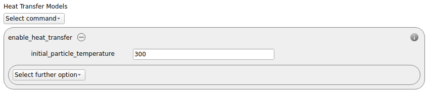
The calculation of the heat transfer is triggered by the enable_heat_transfer command command:

Finally also the gravity is defined:

Per default the gravity has a magnitude of 9.807 and acts into negative z-direction. These defaults can be changed by either setting the magnitude or the direction manually; see enable_gravity command command.

Particles

In this section one sets the material related parameters and defines all particle templates, particle distributions and insertion commands. There is also the possibility to insert single particles or particles arranged in a lattice with the create_particles command command. For postprocessing purposes one can also mark groups of particles for tracking them throughout the simulation.

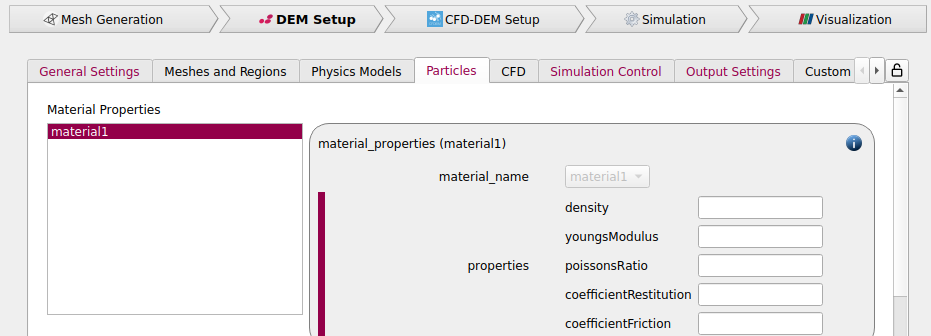
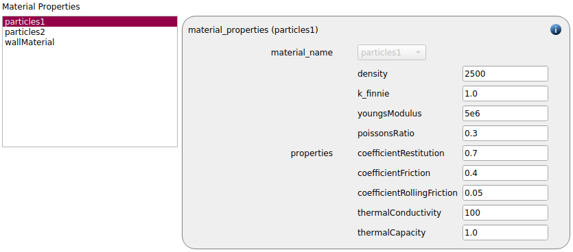
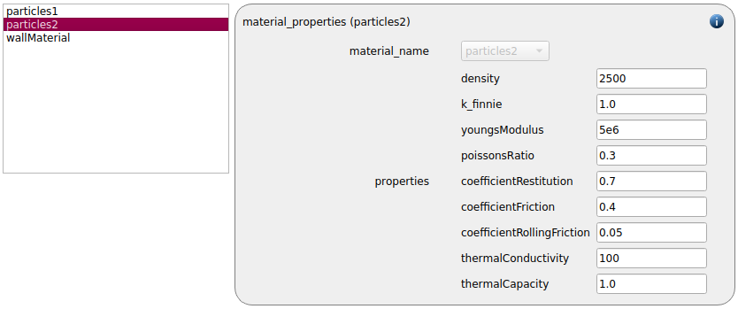
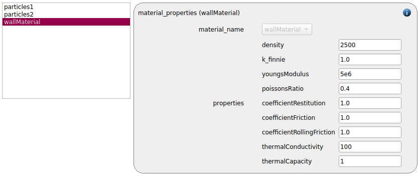
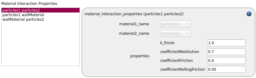
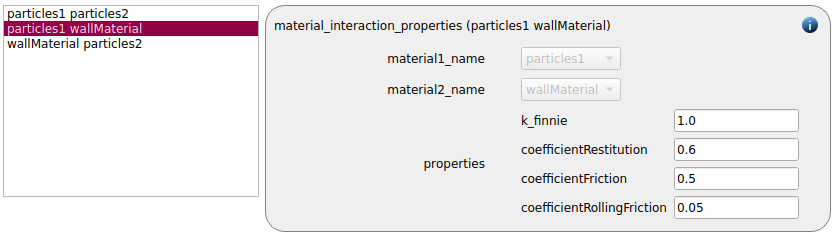
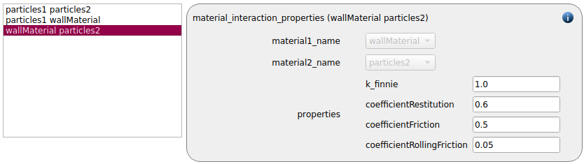
In the general settings tab we only defined three materials, so consequently we have to define the material properties for all materials and the material interaction properties for all possible combinations:

Two particle templates with particles of 3.5 and 5.5 mm radius are generated:

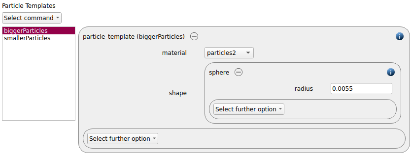
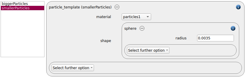
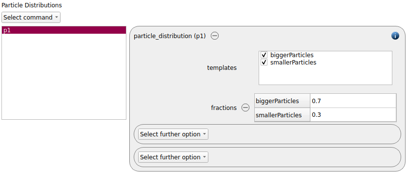
Please note that the smaller particles are of type particles1, while the bigger particles are of type particles2. We use different materials for being able to evaluate the mixing index of the bigger and the smaller spheres. The two templates are used to create a particle distribution that consists of 30% smaller particles and 70% bigger particles:

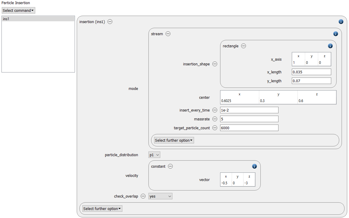
After generating the distribution, a way to insert the particles has to be selected. Here the insertion command command with the mode stream is used. A total of 6000 particles is inserted with a mass rate of 5 kg/s. Particle insertions take place every 0.01 seconds, the initial velocity of the particles is set to (-0.5 0 -3) m/s.

The particles are inserted via a rectangular shape, which is defined within the insertion command.

Coupled simulation

Aspherix® offers the possibility to run one-way coupled calculations against static fluid fields. Both the impact of velocity and temperature fields can be considered. For fully coupled simulations (four-way coupling) Aspherix® has to be coupled against a CFD code that is suitable for coupled calculations (e.g., CFDEM®coupling). All required settings can be made in the CFD tab:

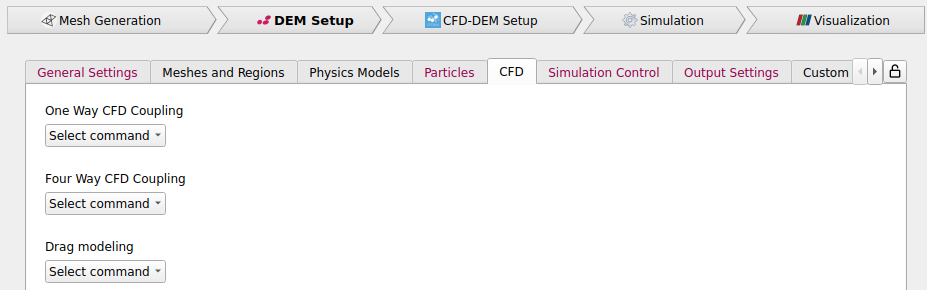
By using the enable_one_way_coupling command command one can either apply a global drag force term or use a velcity field that can e.g., stem from a CFD calculation. In the current example we use a fluid velocity field and apply it to the region region_drag:

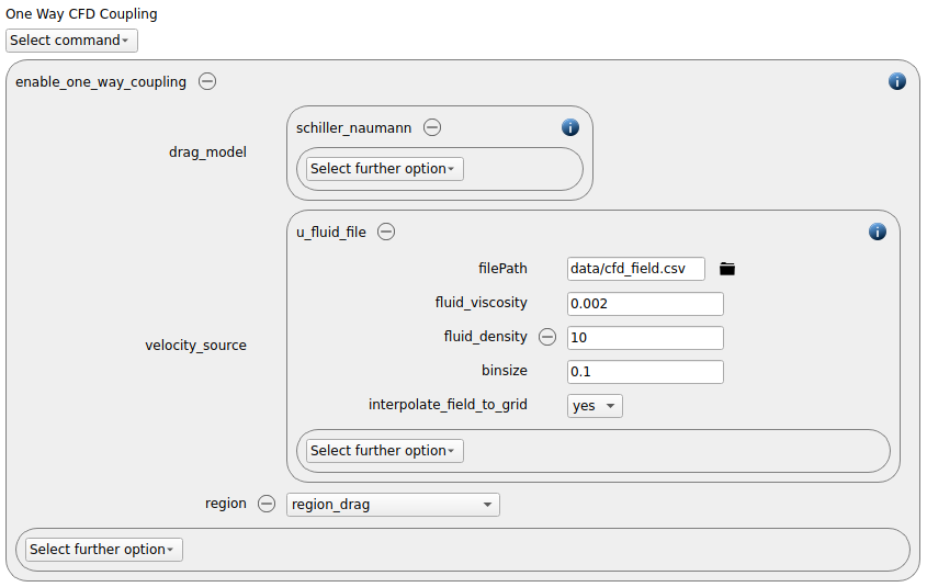
The given field has the following format:

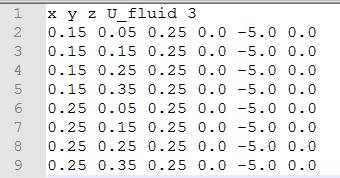
Each of the values gives the coordinates of the center of each cell as well as the velocity.

Velocity fields in csv format can be visualized with the help of Paraview, filters such as tableToPoints and resampleToImage can be used.

Simulation control

All settings that refer to the control of a simulation are made in the “Simulation control” tab. Mandatory setting such as time step width and simulation time can be found here just as well as settings that improve the simulation performance such as load balancing and coarsegraining. The processors command in the “Scalability and speed” section has become obsolete as soon as the loadbalancing command is enabled.

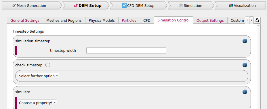
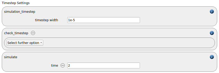
In this tab one first choses the time step settings such as the desired simulation timestep of 1e-5 seconds and the total simulation time of 2.0 seconds. Per default also the check_timestep command command is enabled, which throws a warning when the time step exceeds 10 % of the Rayleigh or the Hertz timestep. These thresholds can be changed by setting an alternative value for hertz_fraction or rayleigh_fraction.

Remark: This tab provides the possibility to define a skin_size and/or a bin_size for the neighbor_list command builds. For most cases (relatively narrow particle distribution, domain-to-particle-size ratio not too large etc.) this setting is not required, but for edge cases this might become important. Generally, the recommended value for the skin size is the average particle diameter, but for edge-cases this can differ. For highly polydisperse particle distribution the best choice depends on the exact case setting.

The enable loadbalancing command is added automatically. When running simulations in parallel, it ensures an optimal distribution of the load on the processors.

Output settings

Writing all desired data in a reasonable frequency is crucial for successful postprocessing. This tab allows the user to define the interval for writing particle data and global information, as well as to use calculate commands for additional evaluations (e.g., center of mass, partile residence time, massflow, …). Please note that the write_to_file command command is a useful tool for writing additional information to files. Currently it can only be used as custom command in the “Custom Settings” section (use file weight 23 and please check the documentation of the command for more details).

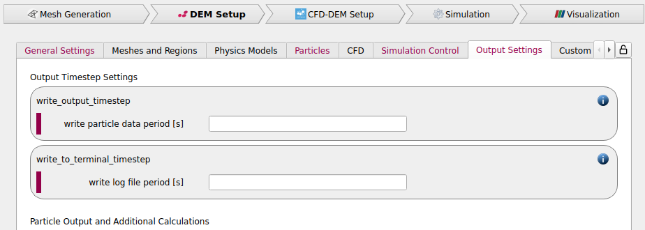
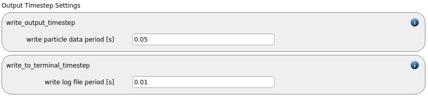
In this tab we first define the timestep width for the file and the terminal output:

The “output_settings” command the takes care that all particle information and the meshes are written to files accordingly. Furthermore it triggers the output of global quantities such as the kinetic energy of the particles or total normal and shear stresses onto meshes in the terminal. As additional output we would like to see the center of mass, the residence time of the particles within the previously defined region, the spatial average and the mixing index. We use additional calculate commands to obtain this output:

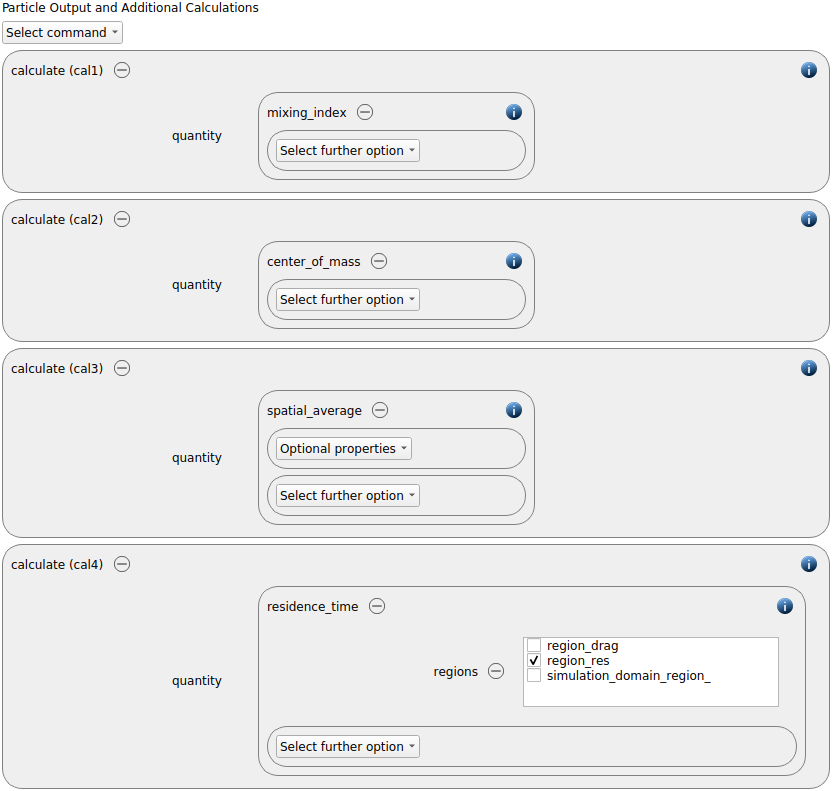
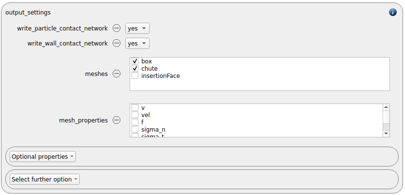
Remark: please note that per default all meshes are written by the output settings, but without potentially available values for stress, wear, velocity etc. Please use the mesh_properties command for producing the desired output. If meshes are added to the meshes list but no mesh_properties are selected, all available properties will be written by default.

The setup of this case is complete now, we can save the setup and move on to the simulate section. The following two tabs are not required for setting up this case, we will only have a brief look there.

Custom settings

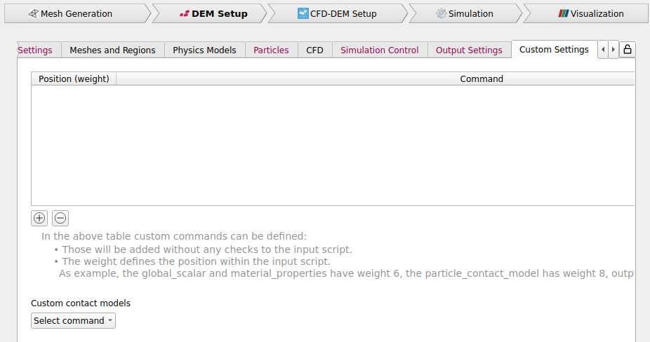
Aspherix® GUI offers a wide range of functionalities, however, for technical reasons it can not cover all possibilites that are provided by Aspherix® Solver. Particularly for advanced users there is the possibility to use Aspherix® Solver commands directly, only a file weight has to be added. If the command is an additional output command, weight 23 is reasonable, integrators should have weight 16. The simulate command has weight 25, so whatever comes afterwards will not be included in the simulation.

Expert settings

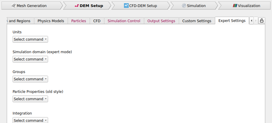
This tab contains commands that should only be changed by experienced users. Particularly when working in this tab, the “Expert Mode” should be activated (View / Expert Mode). In this view some hidden options become visible that are rarely required but can sometimes be helpful.

Running the case

We now change to the simulation view by hitting the Simulation button.

Before launching the actual calculation, a check of the case settings can be performed:

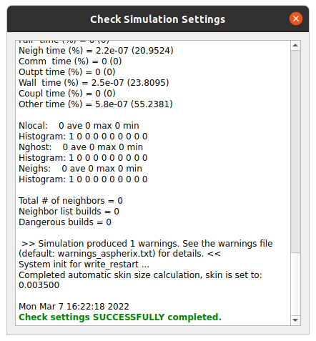
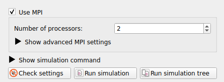
If the test could be completed successfully, this is indicated be the green message Check settings SUCCESSFULLY completed at the bottom of the pop-up window. After closing it again, the real simulation run can be launched by hitting the Start button. One can decide, whether the simulation should be run serially or in parallel and in the latter case the number of processors can be selected:

During the run of the simulation several quantities are displayed. Per default, the number of particles and the translational kinetic energy are displayed:

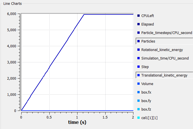
The data displayed in the graph can be edited and saved as image for further usage in reports and presentations for example.

A detailed description of all Aspherix solver commands can be found in the Aspherix solver documentation.

Postprocessing

As soon as data was written to the post-folder within the simulation, it can be displayed with Paraview. Change to the visualization view therefore:

If the simulation has already created output data files and the paths to the Paraview and Ovito are set correctly the results can be visualized with Paraview or Ovito:

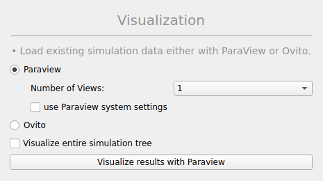
Please launch your preferred postprocessing tool!

Postprocessing with Paraview

When clicking on it, Paraview opens and the data is loaded automatically in four different views:

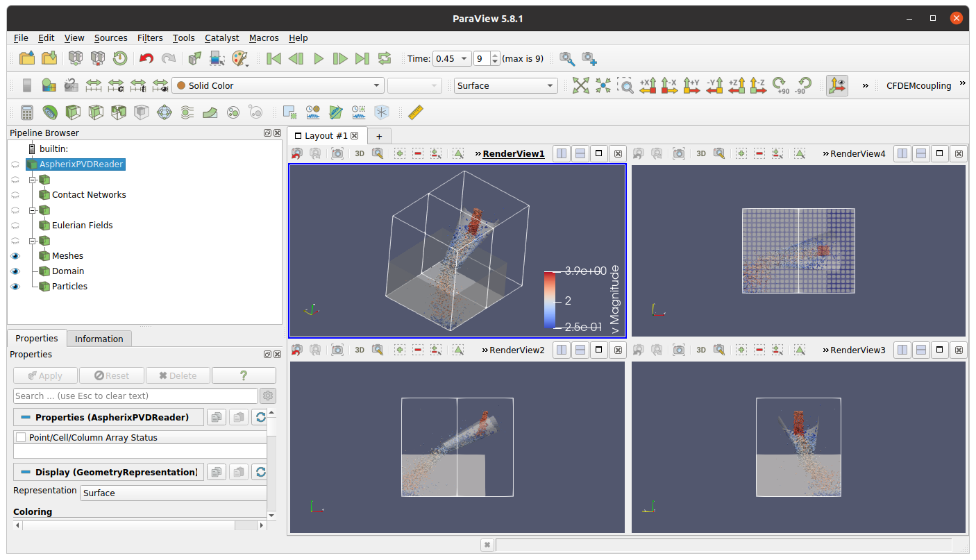
Depending on the availability, the auomatically applied macros extract blocks that contain the particles, the meshes, contact networks, eulerian fields and the simulation.

A few basic steps for postprocessing simulations with Paraview can be found here.

Postprocessing with Ovito

After launching Ovito, all data sets are loaded as separate visual elements. If desired, the user can unite all meshes to a single component (VTM file reader / Unite all meshes).

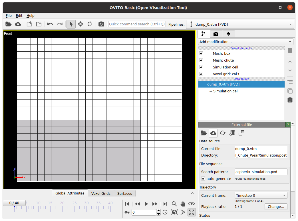
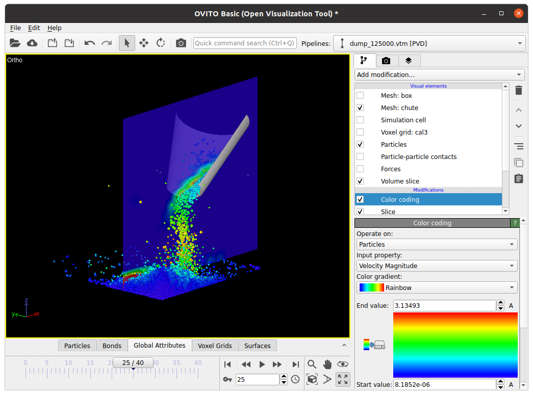
In this case, the eulerian grid data covers the remaining components at startup. By applying modifiers (e.g., Color coding to the particles, a slice to the Particle-particle contacts etc.) one can achieve results as the following:

A few basic steps for postprocessing simulations with Ovito can be found here.