Usage of particle groups

This tutorial deomonstrates different possibilities for using the define_group functionality.

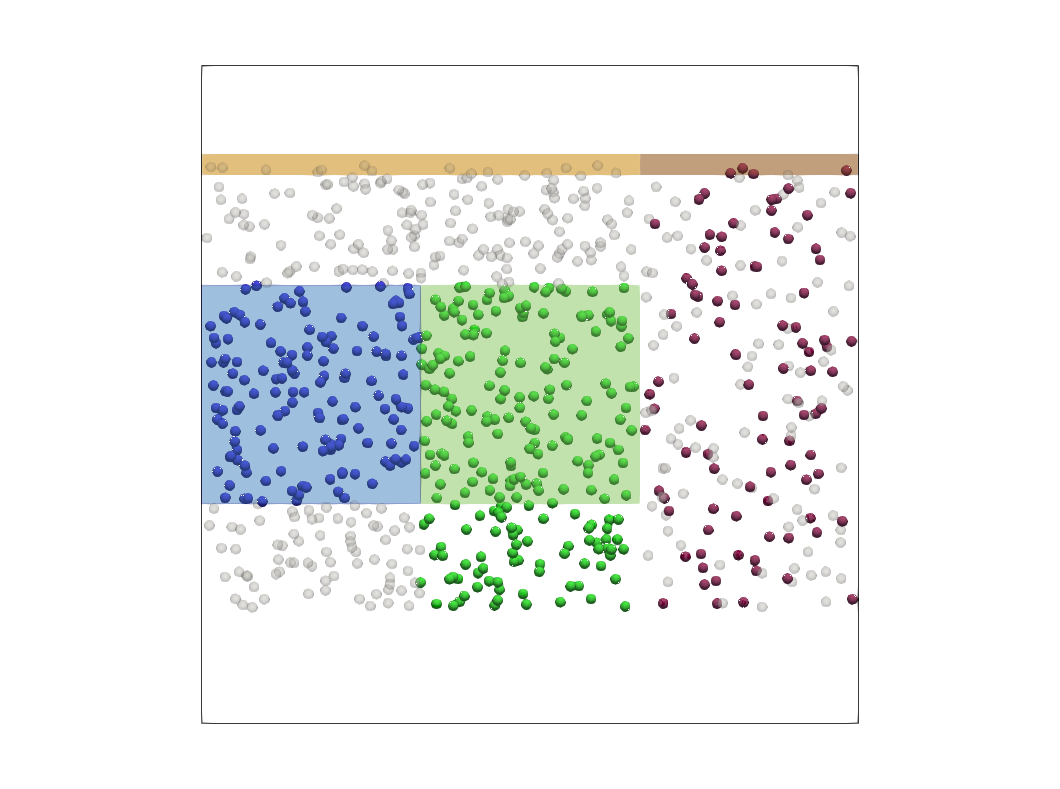
The image shows the overall case setup. Two insertion commands are used to insert continuous streams of particles. The left insertion (light brown) inserts particles from a single material. A non-accumulative define_group command in the blue region adds all particles to the group, that are currently in this region (blue particles). The define_group command that acts in the green region is accumulative, meaning that particles that enter this group remain there (green particles). The right insertion commands inserts particles of two different materials, the second of which is automatically added to a group by a third define_group command (magenta particles).

Name of the case: Project_Particle_Groups

Setting up the simulation

As a first step, the particle shape, the used materials command and the simulation domain are defined in the General Settings tab.

General settings

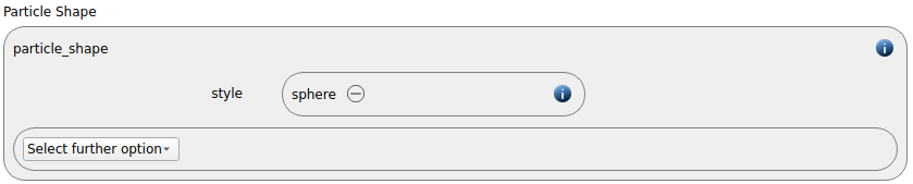
In this simulation we set particles of particle shape sphere:

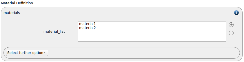
Two materials command “material1” and “material2” are generated:

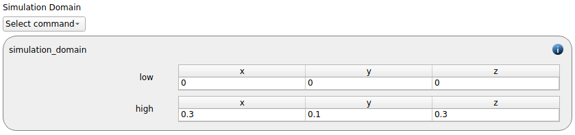
The simulation domain ranging from 0 to 0.3 in x, from 0 to 0.1 in y and from 0 to 0.3 in z direction is created:

Meshes and regions

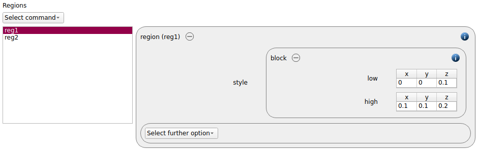
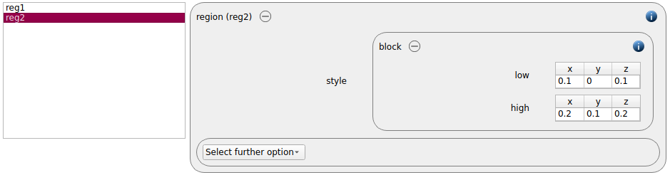
For the backplate, two regions are inserted. Both regions are cubes with a side length of 0.1 meters, one will be used for defining a non-accumulative particle group and one for defining an accumulative one.

Physics models

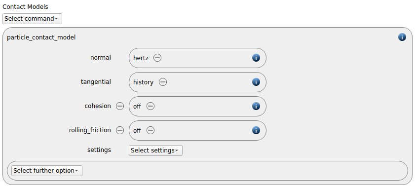
The contact models are now defined. For the particles we use the normal contact model hertz and the tangential model history.

Since this is a very basic test case, the gravity is removed.

Particles

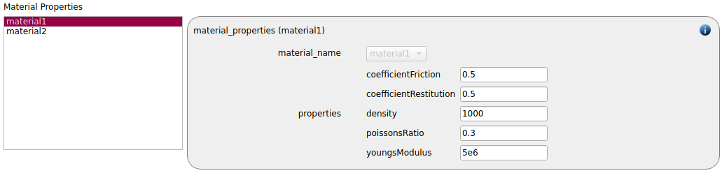
In the general settings tab the material properties are defined:

	material1	material2
Density	1000	1000
Young’s modulus	5e6	5e6
Poisson’s ratio	0.3	0.3
Coefficient of restitution	0.5	0.5
Coefficient of friction	0.5	0.5

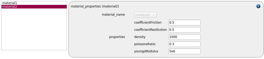
Since two materials are present, also the material interaction properties must be set:

	wall_material - powder
Coefficient of friction	0.5
Coefficient of restitution	0.5

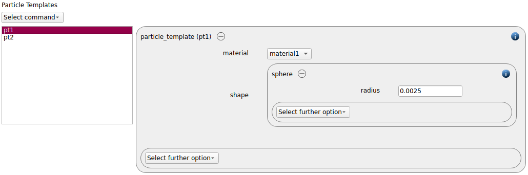
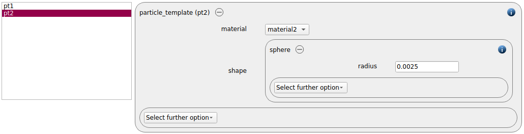
In the next step, two particle templates are defined. For pt1 we use material1, for pt2 we use material2:

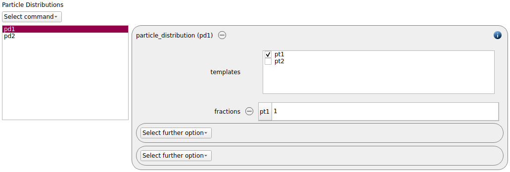
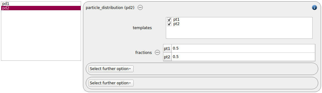
Then, two particle distributions are created. pd1 consists of material1 only while pd2 is a half-half mixture of the two materials:

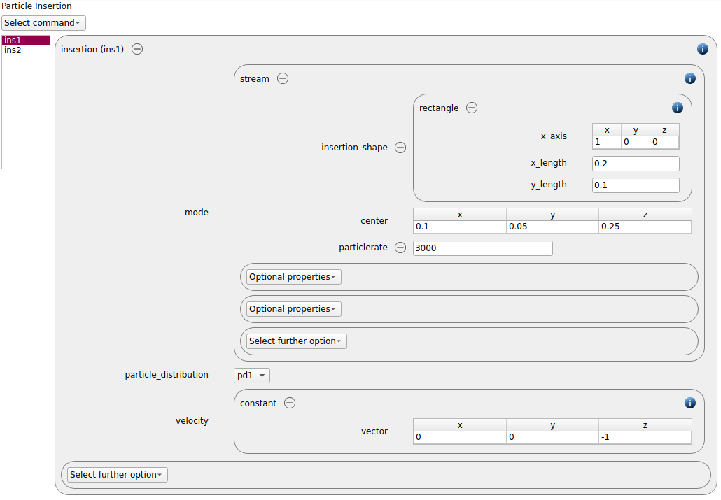
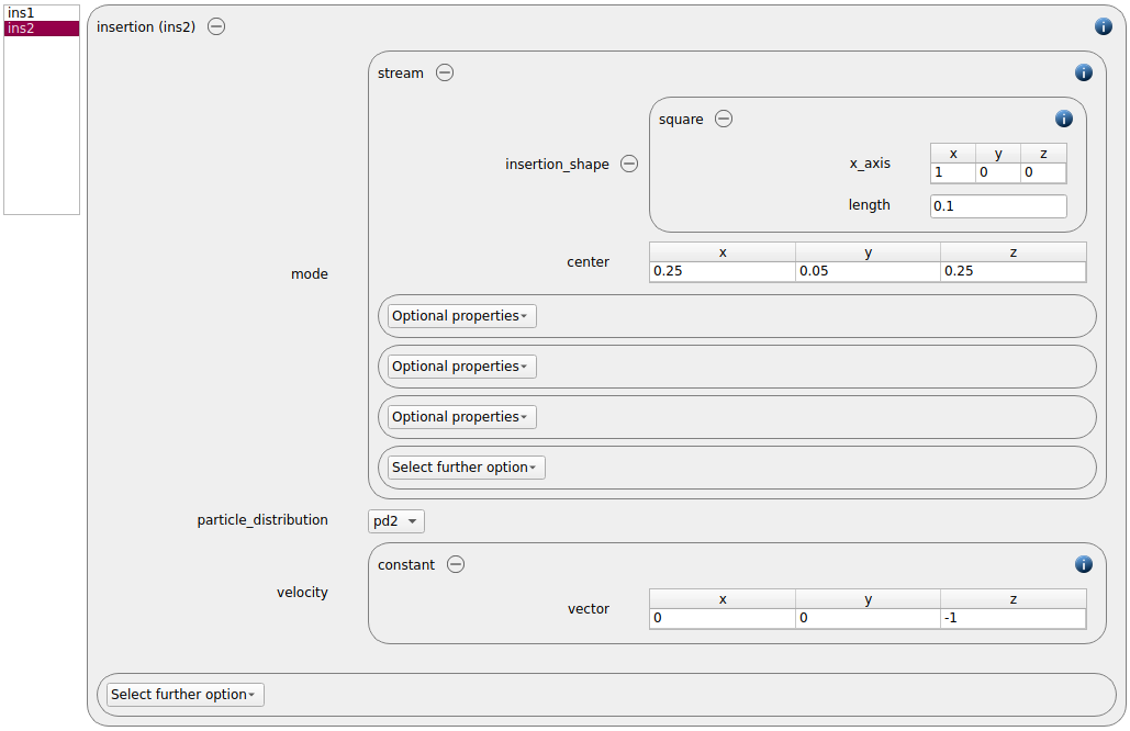
Two insertion command commands are used. In the first one we use a rectangular insertion face to insert a stream of particles using particle distribution pd1. In the second command we use particle distribution pd2. In both cases the particles are inserted with a velocity of 1 m/s in negative z-direction. For the first insertion we use a particle rate of 3000 particles per second, for the second command we stick with the default particle rate.

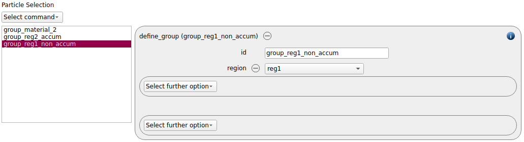
We proceed with the addition of three define_group command commands. First we use the command with its default behaviour (non-accumulative and non-static) and apply it to region reg1:

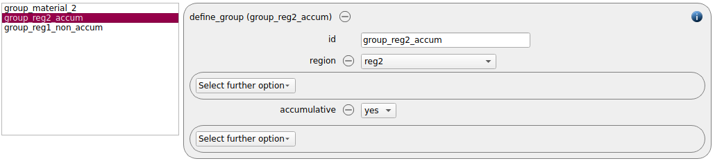
Then we define an accumulative group which is applied in region reg2:

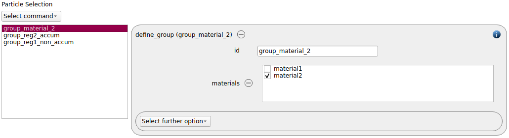
Finally we define a group for material2:

Simulation control

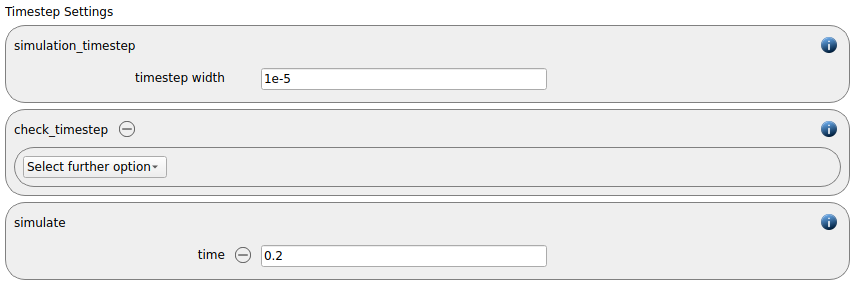
In this tab, we first define the time-step settings such as the desired simulation timestep of 1e-5 seconds and the total simulation time of 0.2 seconds. Per default also the check_timestep command command is enabled, which throws a warning when the time step exceeds 10 % of the Rayleigh or the Hertz time. These thresholds can be changed by setting an alternative value for hertz_fraction or rayleigh_fraction.

We will run this case on a single core, the loadbalancing command can be removed.

Output settings

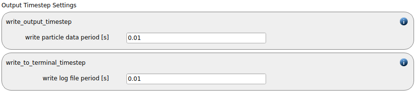
In this tab we first define the timestep width for the file and the terminal output:

The output_settings command command the takes care that all particle information is written to files accordingly. Furthermore it triggers the output of global quantities such as the kinetic energy of the particles to the terminal:

Running the simulation

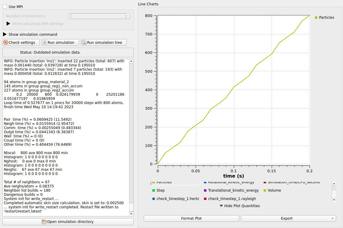
After completing the setup and saving it, the simulation can be launched. It is best to run this small test case on a single core, deactivating the “Use MPI” setting:

Postprocessing with Paraview

After the simulation is completed, all data written with the output_settings command can be visualized automatically by going to the Visualization view and hitting the “Start Paraview” button.

The image below shows the final state of the system:

The image shows the overall case setup. Two insertion commands are used to insert continuous streams of particles. The left insertion (light brown) inserts particles from a single material. A non-accumulative define_group command in the blue region adds all particles to the group, that are currently in this region (blue particles). The define_group command that acts in the green region is accumulative, meaning that particles that enter this group remain there (green particles). The right insertion commands inserts particles of two different materials, the second of which is automatically added to a group by a third define_group command (magenta particles).