The effect of coarsegraining

The amount of computational resources necessary to solve all the degrees of freedom of an industrial-scale application is usually prohibitive due to the enormous amount of particles involved. Coarsegraining is a tool for the reduction of the computational effort by scaling the particle size by a coarsegraining factor. This leads to a decrease of the model size by the factor of cg-factor^3.

However, since the particle size affects the dynamics of the system, it is not possible to simply reduce the particle diameter, as the effect of the particle scaling has to be accounted in all physical models. Some models in Aspherix(TM) already account for coarsegraining, others do not (meaning that they could either be invalid or simply unchecked). All models are aware of whether they account for coarsegraining or not and throw warnings or error messages (depending on the model_check mode) if they do not.

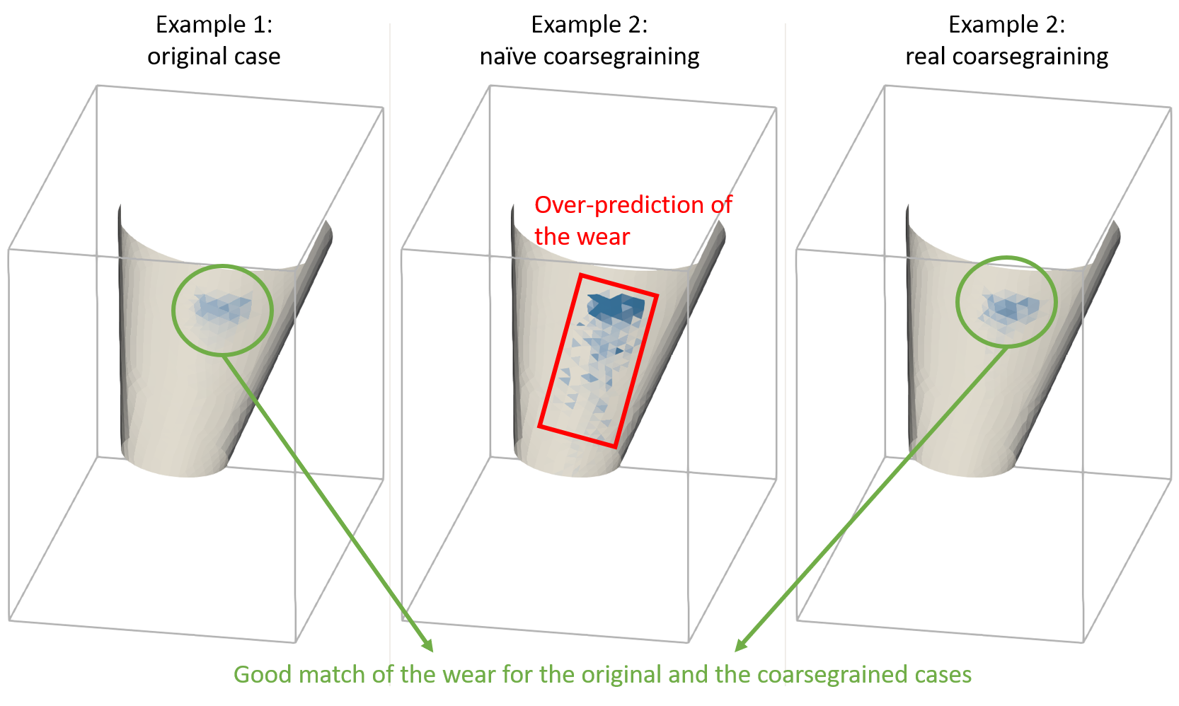
In the following tutorial, three different cases are compared: the first case is the original one, namely some particles are dropped onto a chute on which the wear is calculated. A drag force is applied onto the particles. The second case is identical to the first one, except for the fact that the particle diameter is twice as big. This case represents a so-called “naive coarsegraining”. In the third case, a “real coarsegraining” is used, while the remaining case settings are the same as in the original case.

Name of the case: Project_Coarsegraining

Case 1: “The original”

First, the used materials command as well as the simulation domain are defined in the General Settings tab. Please note that the dimensions of the simulation domain can only be defined in the first simulation. This means that the box that forms the simulation domain has to be chosen big enough from the beginning.

General settings

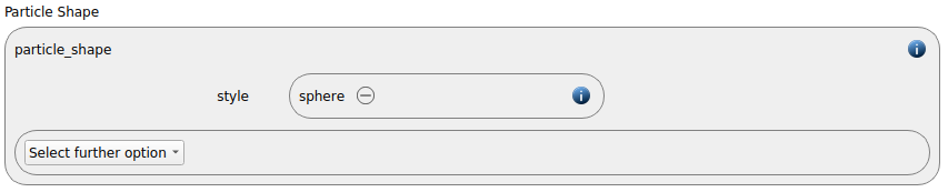
In this simulation we set particles of particle shape sphere:

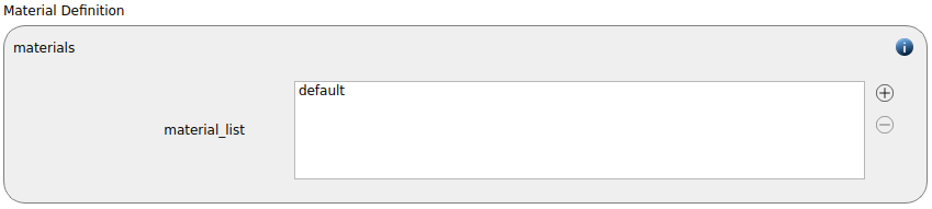
A single materials command with the name default is used:

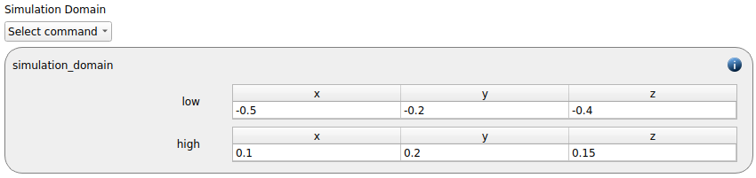
The simulation domain is defined with x dimension ranging from -0.5 to 0.1 meters, y dimension ranging from -0.2 to 0.2 meters and z domain ranging from -0.4 to 0.15 meters.

Meshes and regions

First, we create a mesh module for calculating the wear on the chute:

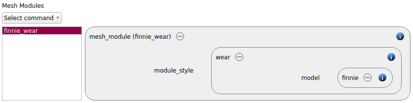
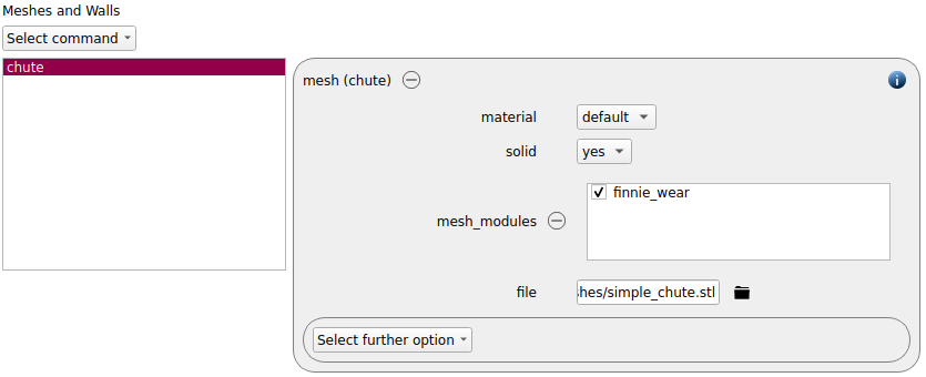
The mesh command command is then used to load the chute geometry and the mesh module “finnie” is activated:

Physics models

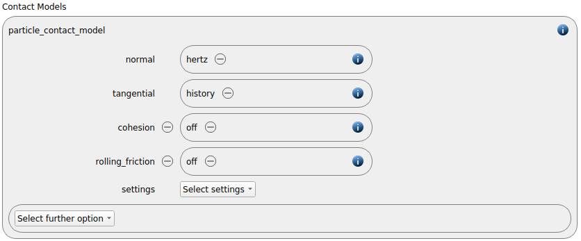
In the next step, the definition of the physics models takes place. For the particles we use the normal contact model hertz and the tangential model history.

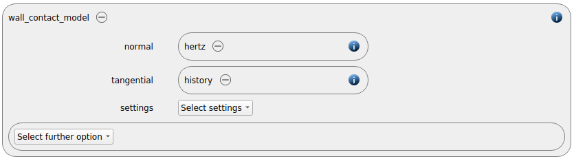
Since a wall mesh (the chute) was added in the previous section, a wall contact model is added automatically in this section. We use the same properties of the particle contact model:

Finally, the gravity is enabled:

Per default, the gravity has a magnitude of 9.807 and acts into negative z-direction. These defaults can be changed by either setting the magnitude or the direction manually.

Particles

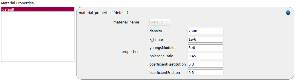
In the general settings tab we only defined a single material type (default), whose settings have to be specified here:

	default
density	2500
k_finnie	1e-6
Young’s modulus	5e6
Poisson’s ratio	0.45
Coefficient of restitution	0.3
Coefficient of friction	0.5

Please note that the required property for the wear model (i.e., the Finnie constant k) was added automatically when selecting the wear model for the wall.

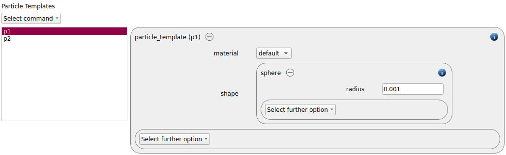
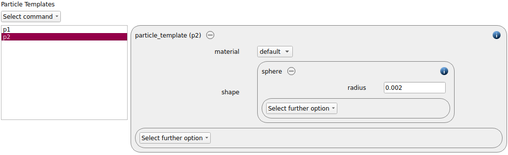
Two templates for spheres with radii of 0.001 and 0.002 meters are generated:

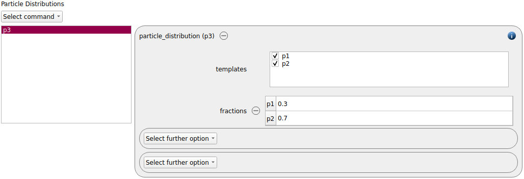
Based on these templates, a particle distribution is created:

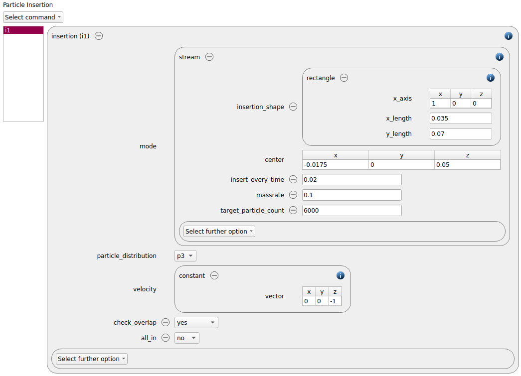
The final step in this tab is the definition of the insertion command. We use mode stream to add a maximum number of 6000 particles with a mass rate of 0.1 kg/s. Please note that the definition of a mass rate instead of a particle rate is crucial in this case, since the number of particles will be reduced later on via coarsegraining. The initial velocity of the particles is given with (0,0,-1) m/s. The insertion is done through a rectangular insertion_shape normal to the x axis, centered at (-0.0175, 0, 0.05) and with lengths of 0.035 and 0.07 in the x and y directions, respectively. Particles are inserted every 0.02 seconds. Furthermore the overlap check was set to yes (this is the default value), all_in is set to no.

Coupled simulation

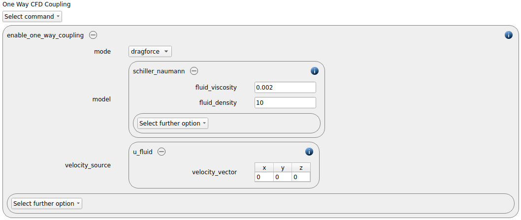
In the next step, a drag force is defined to act onto all particles in the simulation domain. A Schiller Naumann model is used with a viscosity of 0.002 m^2/s and a density of 10 kg/m^3. A velocity source is required for the drag force, but since we only want the drag effect from the falling particles, all components of the velocity vector are set to zero.

Simulation control

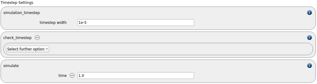
In this tab, one first choses the time step settings such as the desired simulation timestep of 1e-5 seconds and the total simulation time of 1.0 second. Per default, the check_timestep command command is also enabled, which throws a warning when the time step exceeds 10 % of the Rayleigh or the Hertz time. These thresholds can be changed by setting an alternative value for hertz_fraction or rayleigh_fraction.

Output settings

In this tab, we first define the timestep width for the file and the terminal output:

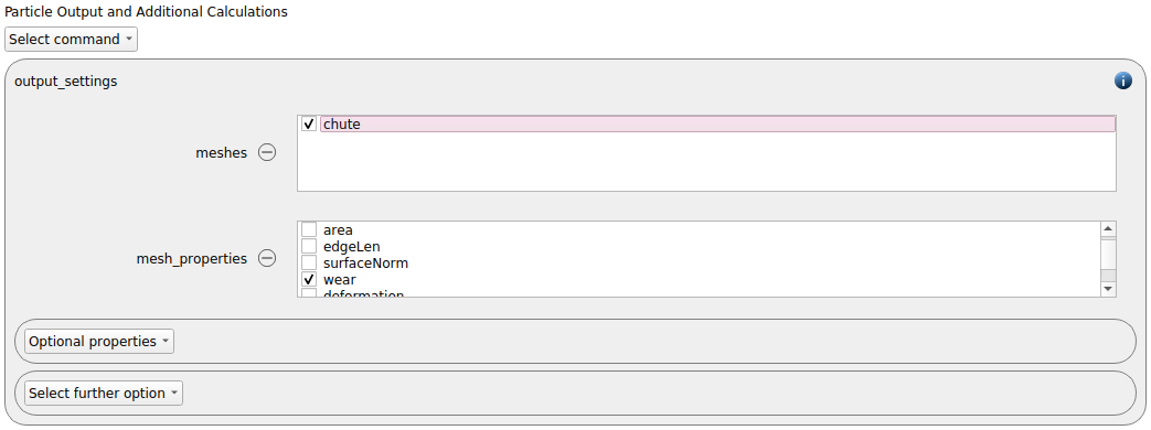
The output_settings command command takes care that all particle information and meshes are written to files. Furthermore, it triggers the output of global quantities such as the kinetic energy of the particles or total normal and shear stresses onto meshes to the terminal. Please note that if the output of per-cell information on meshes such as wear, velocity of stress are desired, one has to add the keyword mesh_properties and select the required output.

Simulation

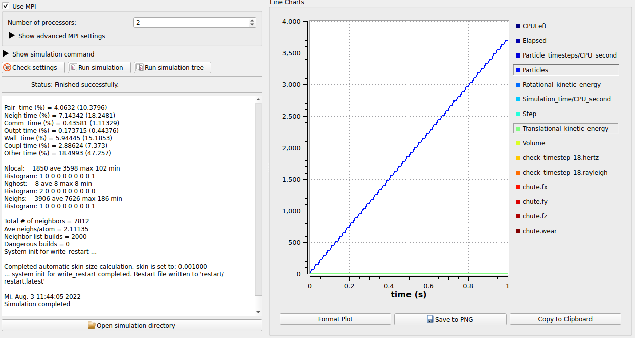
After completing the setup and saving it, the simulation can be launched. Therefore, change to the Simulation view. First hit the “Check settings” button, and if the check returns “Check settings successfully completed” the simulation can be run by hitting “Start”:

Case 2: “Naive coarsegraining”

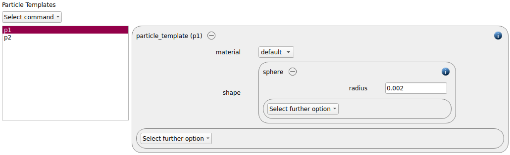
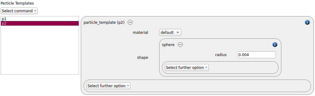
A rather naive attempt of reducing the number of spheres in a simulation would be the increase of the particle radius, while all other quantities remain the same. First, make a copy of the original case using the “Clone simulation” functionality in the context menu and then go to the Particles tab and change the particle radii from 0.001 and 0.002 m to 0.002 and 0.004 m:

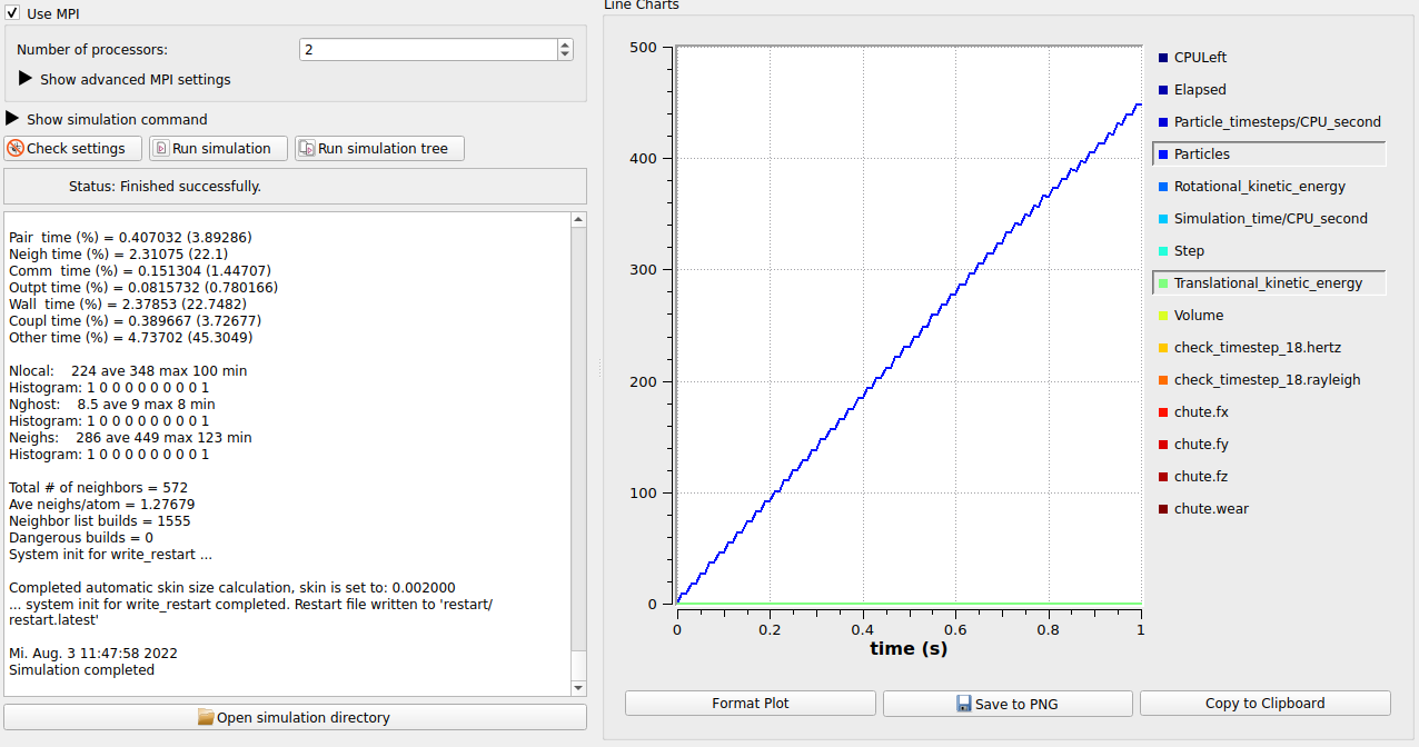
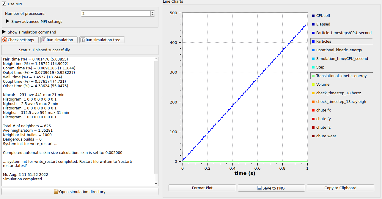
The first difference becomes clearly visible when running the case. Instead of approximately 3800 particles, just around 450 particles are inserted:

Case 3: “Real coarsegraining”

Finally, for preparing the last case, make another copy of the original case using the “Clone simulation” functionality in the context menu. All existing settings remain and coarsegraining will be applied. Go to the Simulation Control tab and select coarsegraining command in the Scalability and Speed section. For making sure that you get a warning instead of an error message when you use models which are not adapted for coarsegraining, select the model_check warn option:

Also in this case, the number of particles in the system is reduced approximately by the factor of 8 (2^3):

Comparison of the results

When comparing the results, it becomes visible that the wear results for the original and the coarsegrained case match quite well, while there is a significant deviation for the case of the “naive coarsegraining”.