Angle of Repose

This tutorial consists of three connected simulations: in the first step a particle bed is generated, secondly a ring is lifted in order to start the formation of the heap and in the last simulation the final settling takes place.

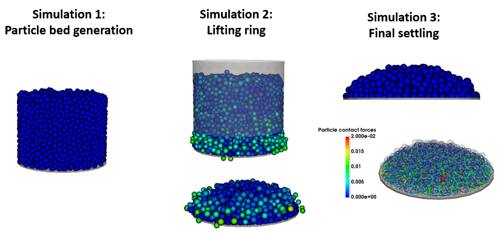
Discussed features are the derivation of dependent simulations, the usage of meshes and primitives as walls, cohesion and the usage of regions for insertion.

Name of the case: Project_Angle_of_repose

Initialization of the particle bed

First of all we start with generating a new project and adding the first simulation:

General settings

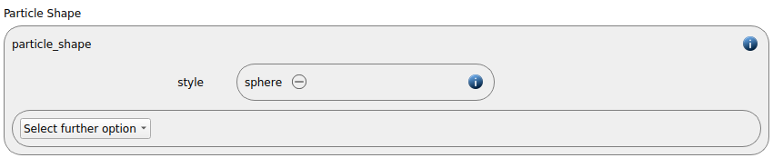
In this simulation we select particles of particle shape sphere:

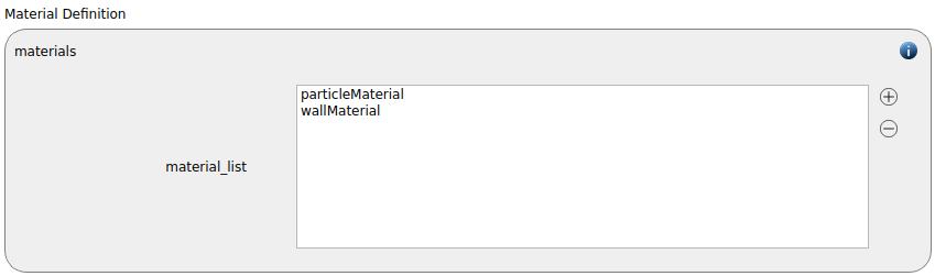
In the current simulation two material types will be used, one for the particles and one for the wall:

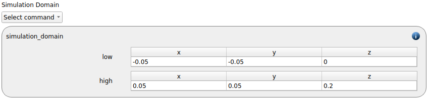
A simulation domain with x and y dimensions ranging from -0.05 to 0.05 and z dimension ranging from 0 to 0.2 is created:

Loading meshes and creating regions

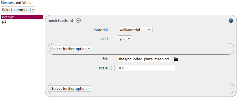
In the current example a round plate with a small fillet at the edge will be used as base plate. The mesh named bounded_plate_mesh.stl is inserted using the mesh command command and scaled with the factor 0.5:

As boundary for the particles during the insertion we use a cylindrically shaped primitive wall:

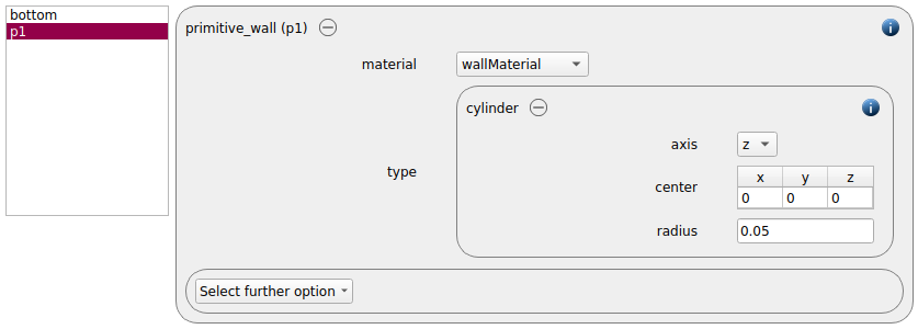
In both cases the material type wallMaterial should be selected.

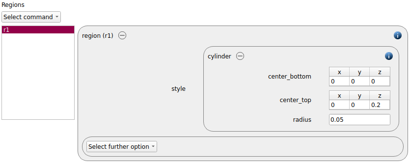
In this case the particles will be inserted in a cylindric region command that has the height of the simulation domain and whose radius is 0.05:

Both objects - the plate and the cylinder - are visualized in the graphics pannel. Please always make sure that all used meshes are inside the simulation domain.

Physics models

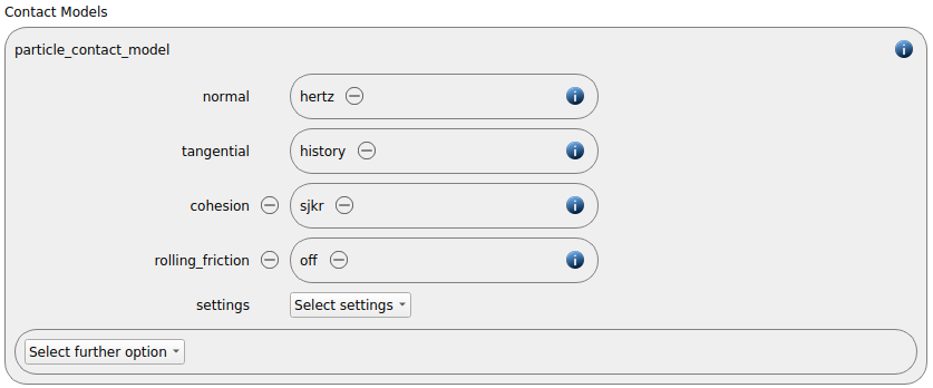
In the next step, the definition of the physics models takes place. For the particles we use the normal contact model hertz and the tangential model history. Furthermore the sjkr cohesion model is selected:

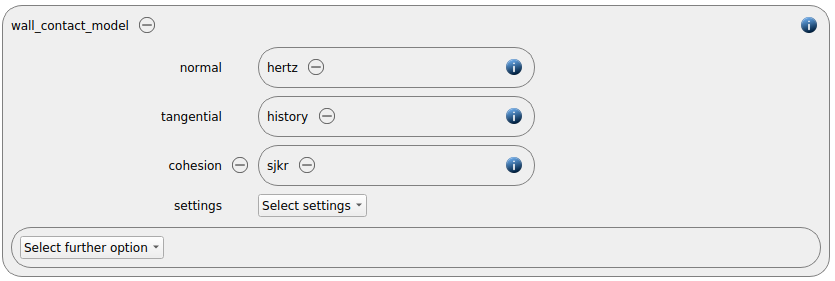
Since we added a mesh and a primitive wall in the previous section, a wall contact model was added automatically in this section. We use the same properties as for the particle contact model:

Finally also the gravity is defined:

Particles

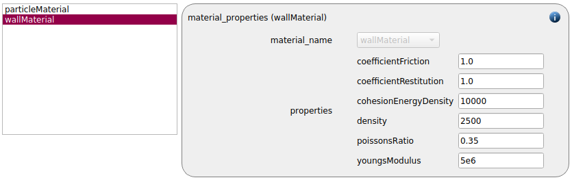
In the general settings we defined two materials, and in this section we have to define their model and interaction properties:

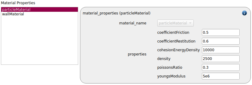
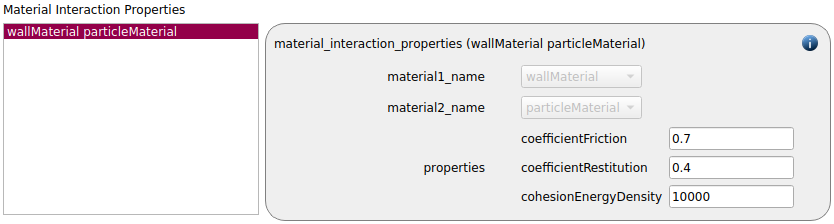
	particleMaterial	wallMaterial
Young’s modulus	5e6	5e6
Poisson ratio	0.3	0.35

	particle/particle	particle/wall	wall/wall
Coefficient of restitution	0.6	0.4	1.0
Coefficient of friction	0.5	0.7	1.0
Cohesion energy density	10000	10000	10000

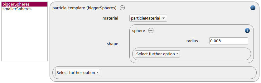
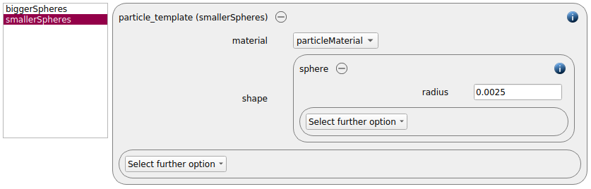
Two templates for spheres of the same material but with different radii (0.0025 m and 0.003 m) are then generated:

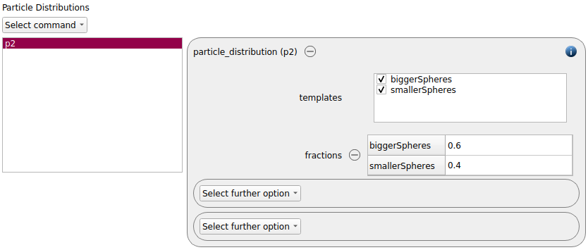
From the two templates a discrete particle distribution is created that consists of 40% smaller and 60% larger particles:

A pack of particles with a velocity of 1.0 m/s in negative z-direction is inserted using an insertion command command with mode pack:

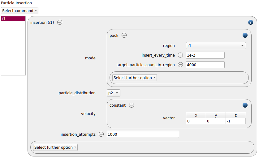
The amount of particles (4000 in total) inserted in the region is rather high in comparison to the available volume, thus the number of insertion attempts (maxattempt) is increased to 1000. Both the keywords check_overlap and all_in are set to yes.

Simulation control

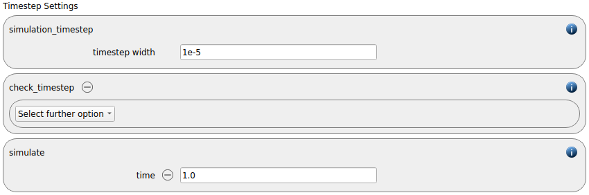
In this tab one first choses the time step settings such as the desired simulation timestep of 1e-5 seconds and the total simulation time of 1 second. Per default also the check_timestep command command is enabled, which throws a warning when the time step exceeds 10 % of the Rayleigh or the Hertz time. These thresholds can be changed by setting an alternative value for hertz_fraction or rayleigh_fraction.

Output settings

In this tab we first define the timestep width for the file and the terminal output:

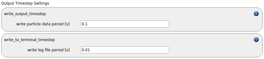
The output_settings command command takes care that all particle information and the meshes are written to files accordingly. Furthermore it triggers the output of global quantities such as the kinetic energy of the particles or total normal and shear stresses onto meshes in the terminal. Please note that if the output of per-cell information on meshes such as wear, velocity of stress are desired, one has to add the keyword mesh_properties and select the required output.

Running the simulation

After completing the setup and saving it, the simulation can be launched. Therefore change to the Simulation view. First of all, use the Check settings functionality to make sure that the setup works:

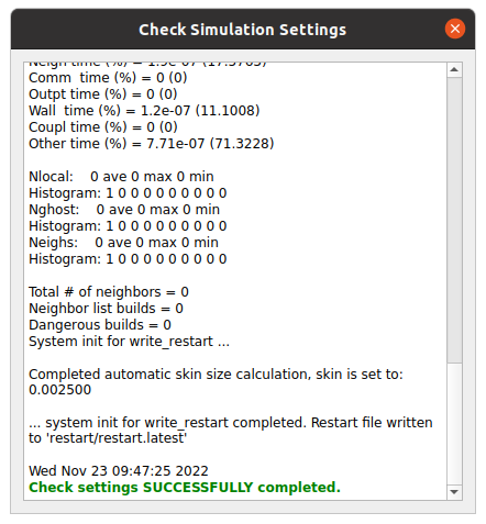
Before running the simulation, you need to chose whether to run it in parallel or in serial and, if in parallel, the number of processors to employ. After hitting the Start button, the simulation is launched. The number of particles, as well as the kinetic energym is displayed in the graphical window, while other quantites can be shown or hidden as well:

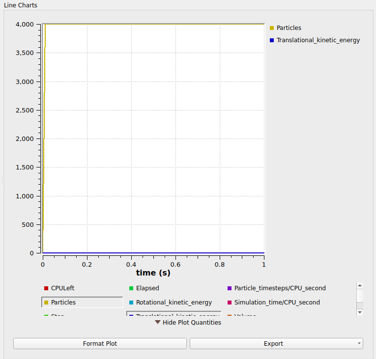
The displayed window offers the possibility to abort the simulation, for example if you notice an undesired behaviour. Please note that in that case the simulation has to be restarted from the beginning, as a restart from the current time step is not possible. When the simulation is completed, one can use Paraview to visualize the results:

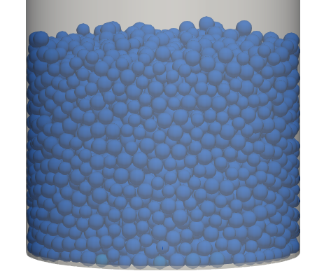
The generated packing looks as desired and one can now proceed with the next simulation.

Lifting the ring

By hitting the “Derive simulation” button below the simulation one obtains a new simulation which contains most of the settings of the previous one. Please note that such a deviation leads to a freeze of the original simulation, meaning that it cannot be modified from that point on. Only the deletion of the derived simulation would make the original simulation modifiable again.

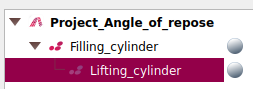
The main difference is that the new simulation uses the data produced in the parent simulation as starting point for the new calculations.

The general settings remain the same, thus one can directly proceed to the meshes tab.

Inserting meshes

In this section we want to replace the previously-defined primitive wall cylinder by a cylindric mesh which is moved upwards. We start with the definition of a motion by adding a mesh module of type motion:

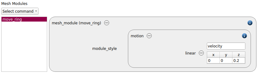
In the surface meshes section the primitive wall can be removed and the cylindric mesh is added.

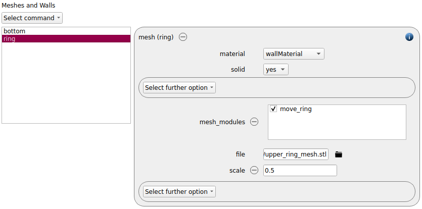
The material type has to be set to wallMaterial and the geometry has to be scaled with the factor 0.5. The correctly scaled mesh can immediately be reviewed in the graphics pannel.

Removing particle insertion and insertion region

As the desired amount of particles has been inserted in the previous calculation, the insertion operation can be removed from this calculation. This also makes the insertion region obsolete. The removal of components has to follow a top-down approach, meaning that commands can only be removed if nothing depends on them. We thus start by deleting the insertion command from the Particles tab first by clicking on the minus next to the command. After this one can proceed with first deleting the particle distribution and then the two particle templates. This leaves a rather empty particles tab, apart from the material and material interaction properties. The definition of the material properties is still required and these quantities can still be changed in a derived simulation. As the insertion command was deleted, one can now also go to the Meshes and Regions tab and remove the cylindric insertion region.

Simulation control

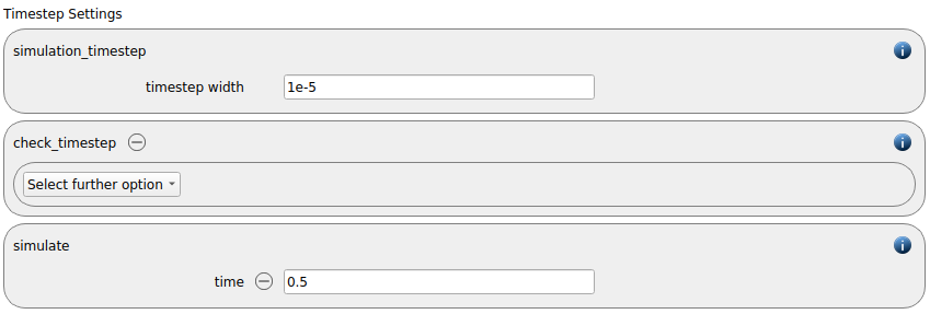
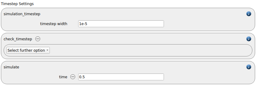
As the lifting of the cylinder will not take as long as the generation of the particle bed, one can reduce the simulation time from 1 to 0.5 seconds:

WARNING: if a mesh leaves the simulation domain during a calculation, an error will occur and the simulation will be aborted.

Output settings

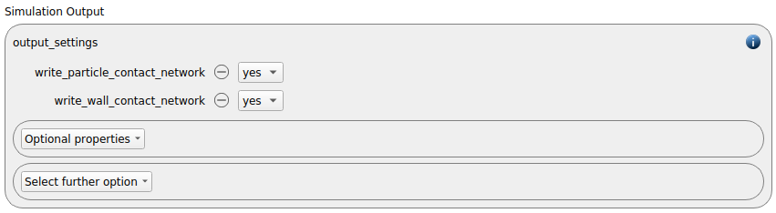
In the output settings we add the keywords write_particle_network and write_wall_contact_network. This enables us to visualize the contacts between particles and walls later on.

Running the simulation

Ths settings are now completed and the simulation can be started:

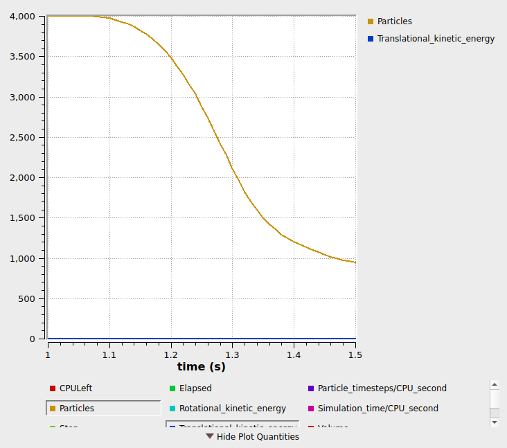
One can see that the number of particles decreases as particles are deleted when leaving the simulation domain. The results can again be visualized in Paraview:

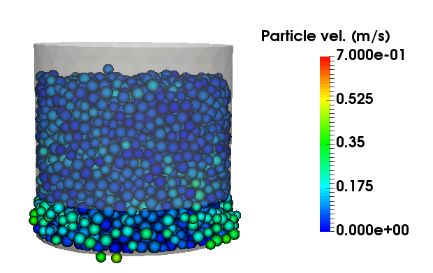
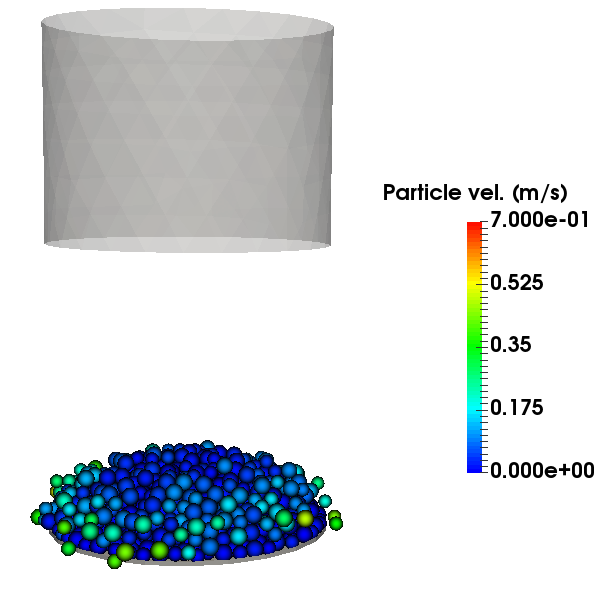
The last image shows that the particles are still in motion and that the settling is not yet completed. One can thus derive a third simulation without the ring, during which the process can be completed.

Final settling

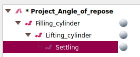
For deriving another simulation one hits the Derive simulation button underneath the previously derived simulation. The Lifting_cylinder simulation is now frozen as well and a new simulation appears in the timeline. The new simulation is renamed into Settling:

Removing the ring

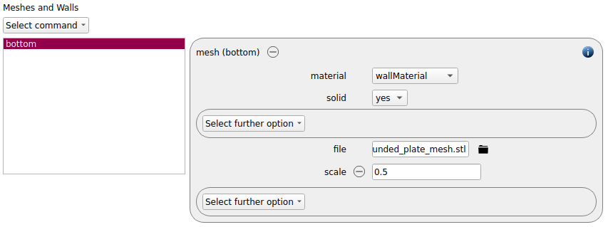
The main change in this case is the removal of the ring. Therefore go to the meshes tab and remove the mesh ring and the mesh module move_ring in this order. The tab now only contains the mesh command command for the base plate:

Simulation control

Just as in the previous case we chose a simulation time of 0.5 seconds:

Output settings

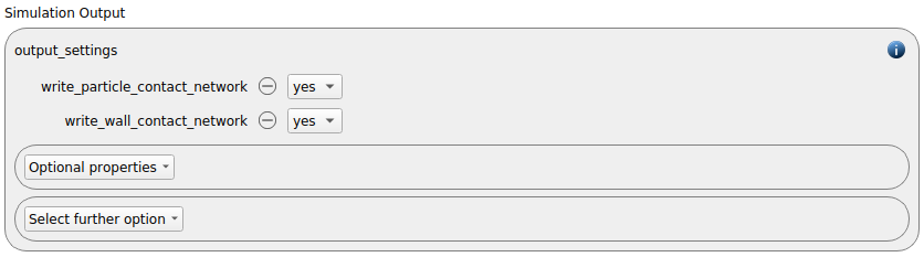
For being able to visualize the contact forces in Paraview, we again select the keywords write_particle_contact_force_network and write_wall_contact_force_network in the output settings.

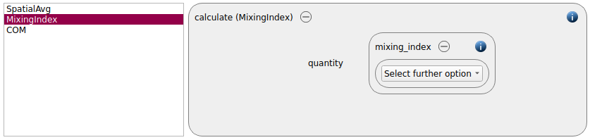
Additional calculations such as the mixing index, the center of mass and the spatial average are added:

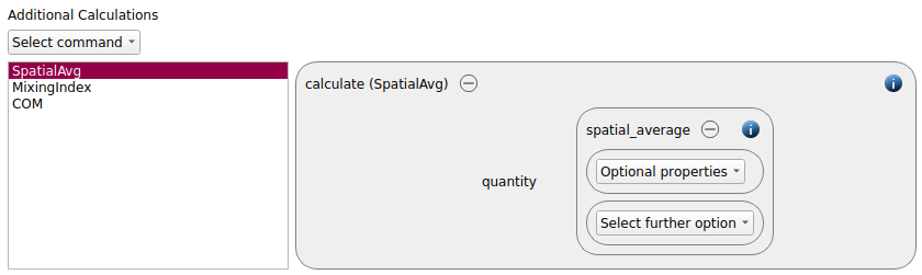
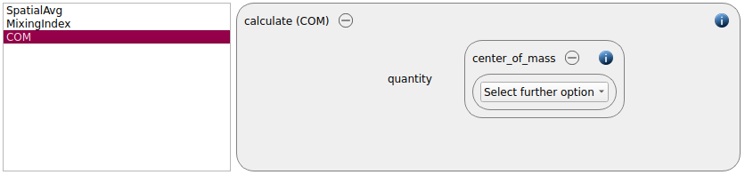
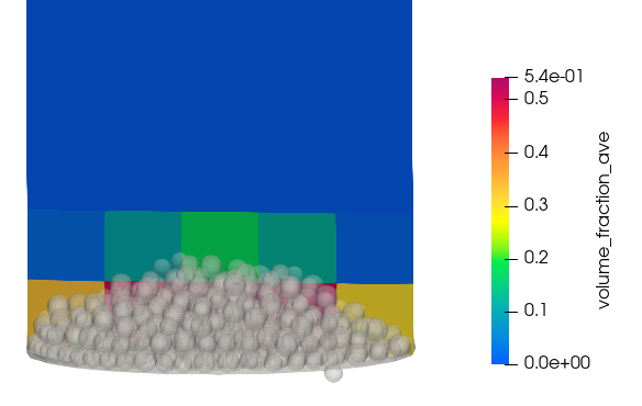
The center of mass option leads to the output of a text-file, while the spatial averaging command leads to a vtk-file.

Running the simulation

As the simulation setup is completed with that step, one can launch the calculation. As can be seen in the graph, the number of particles still increases in the beginning, but then reaches a steady state.

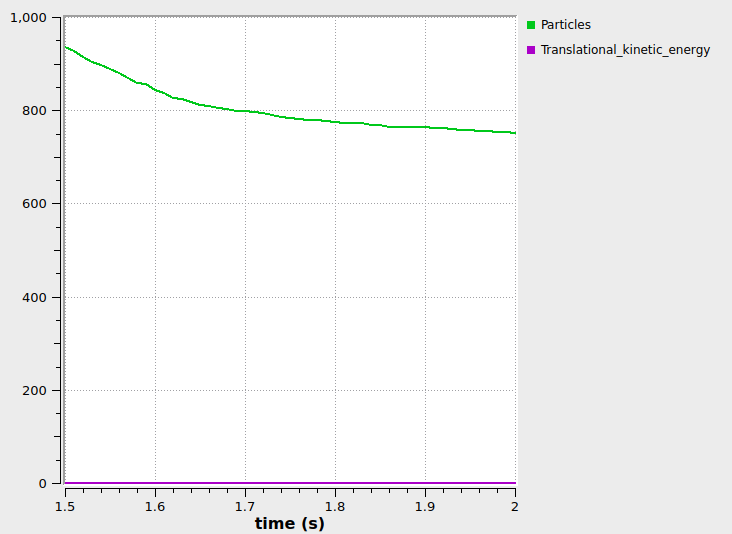
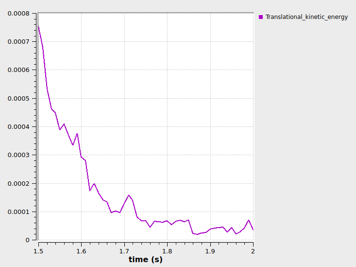
If one deselects Atoms and only displays the kinetic energy, it shows that this quantity goes to zero, indicating that the settling process is completed:

Results

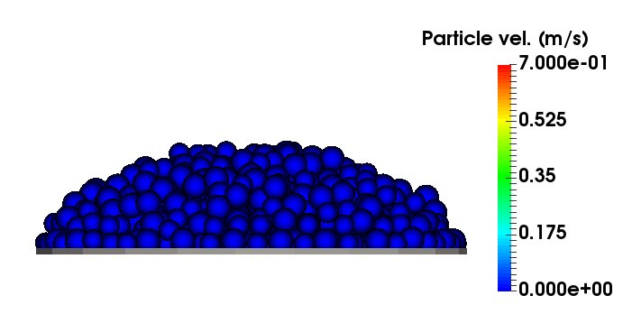
The result can again be visualized with Paraview. One possibility is displaying the particles, coloring them according to the radius or velocity:

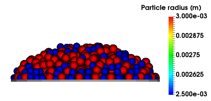
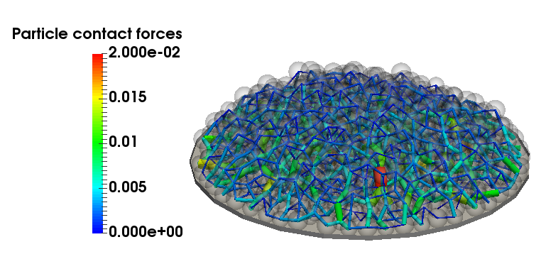
As the particle-particle and particle wall data was written to files as well, one can also display the forces that act between the particles for example:

The result of the spatial averaging is written to the main simulation output file and can directly be visualized in Paraview, the respective component is called “Eulerian Fields”. The below image shows a slice of the average volume fraction field:

The center of mass of the particles can be visualized in the Line Charts window directly:

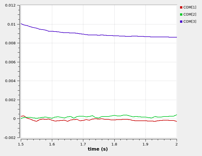
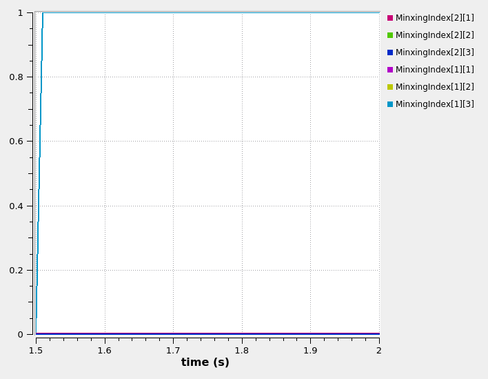
Inside the simulation folder one can also find text files that contain the data for the center of mass and the mixing index (in this case data_COM.txt and data_MixingIndex_material_0.txt and data_MixingIndex_material_1.txt).