Basic DEM Tutorial

This basic tutorial case treats topics such as particle insertion, the usage of a mesh as a physical wall and the presence of gravity: a continuous stream of spherical particles is inserted at a specific initial velocity, the particles start to settle under the influence of gravity and a chute redirects the flow.

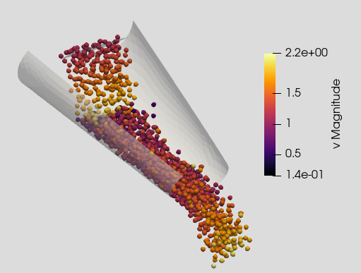
Name of the case: Project_Chute

Simulation setup

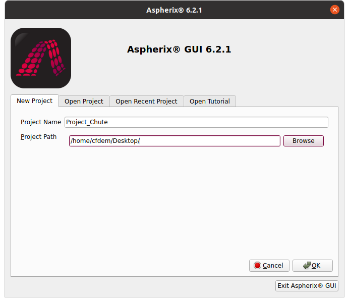
After launching Aspherix® GUI we start with generating a new project at a location of our choice:

General settings

In the General Settings tab particle shape, the materials and also the simulation domain are defined.

We start with setting the particle_shape command type to sphere:

We will use a single material for walls and particles in this case:

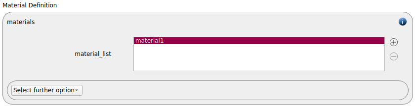
Please note that all materials that are intended to be used in a simulation have to be defined right away, even when some of them are inserted at a later point in the simulation tree.

The simulation_domain command with x dimensions ranging from -0.05 to 0.5 m, y dimensions ranging from -0.25 to 0.25 m and z dimensions ranging from -0.1 to 0.35 m is created:

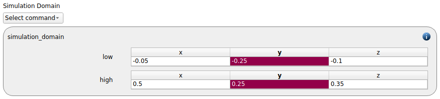
The dimensions of the simulation domain are chosen in dependence of the mesh that is inserted in the next step.

Meshes and regions

We use a prepared chute-geometry (stl-file) as mesh command:

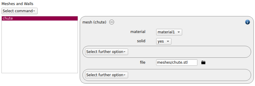
Per default, the option solid yes is added. If a mesh is meant for insertion or massflow measurement, please change this setting to solid no.

Physics models

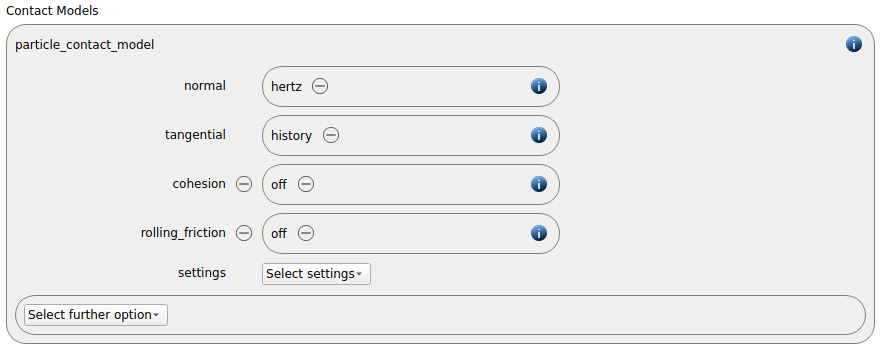
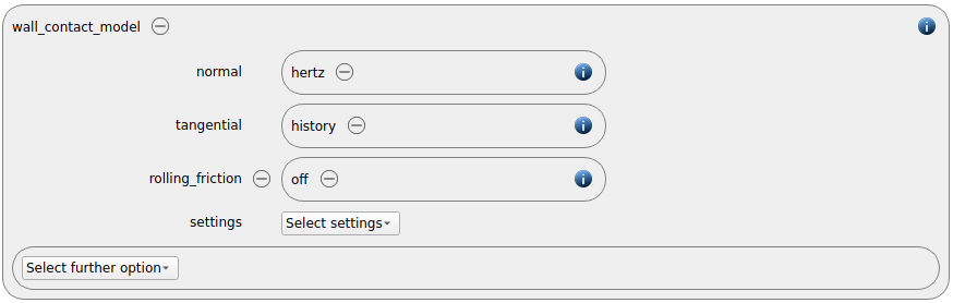
In this tab contact models and other physical models are selected. The particle_contact_model command command is obligatory in all cases, the wall_contact_model command command is added automatically, as soon as a mesh command or a primitive wall is present.

We keep the default settings, namely the normal model hertz and the tangential model history for particles and walls:

The gravity command is added automatically:

Per default the gravity has a magnitude of 9.807 and acts into negative z-direction. These defaults can be changed by either setting the magnitude or the direction manually.

Particles

In this section one sets the material related parameters and defines all particle templates, particle distributions and insertion commands.

All parameters required by contact models and other physical models in the simulation are automatically added as material properties. In this case the following settings must be made:

Parameter	Value
Coefficient of friction	0.4
Coefficient of restitution	0.7
Density	2500
Poissons ratio	0.3
Youngs modulus	5e6

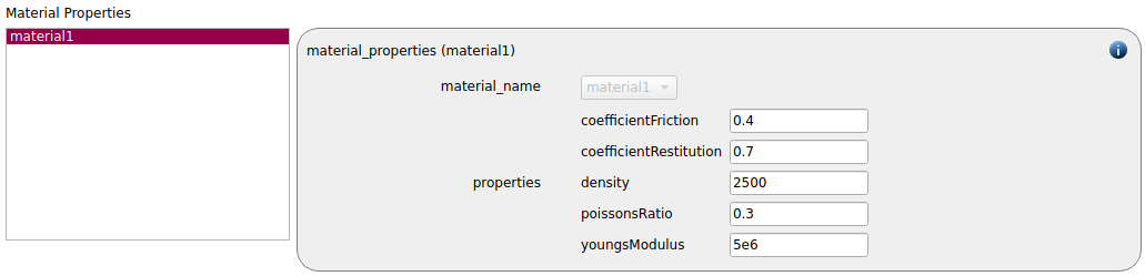
Density, Poissons ratio and Youngs modulus and the coefficient of restitution are material properties that can be measured directly or taken from literature. The coefficient of friction is a bulk property that also depends on factors such as particle shape, surface roughness, particle distribution etc. and can be determined by material calibration.

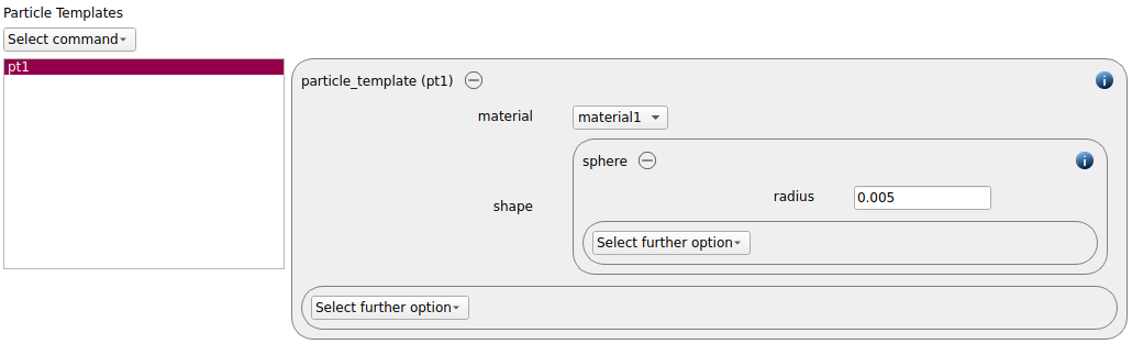
A particle template for spheres with a radius of 5 mm is generated:

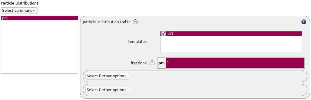
This template is used to define a particle distribution:

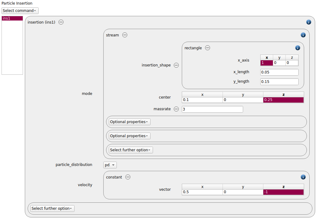
After generating the distribution, a way to insert the particles has to be selected. An insertion command command with the mode stream is used for continuous particle generation with a mass rate of 3 kg per seconds. The initial velocity of the particles is set to (0.5 0 -1) m/s. The particles are inserted via a rectangular shape:

Simulation control

All settings that refer to the control of a simulation are made in the “Simulation control” tab. Mandatory setting such as time step width and simulation time can be found here just as well as settings that improve the simulation performance such as load balancing and coarsegraining. The processors command in the “Scalability and speed” section has become obsolete as soon as the loadbalancing command is enabled.

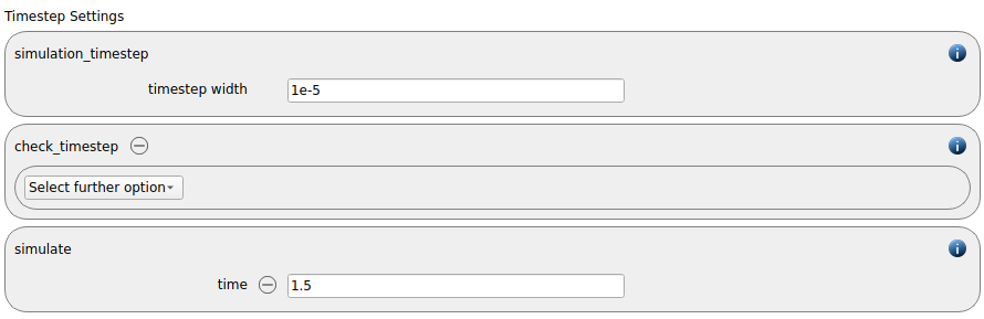
We first define the time step settings such as the desired simulation timestep of 1e-5 seconds and the total simulation time of 1.5 seconds. Per default also the check_timestep command command is enabled, which throws a warning when the time step exceeds 10 % of the Rayleigh or the Hertz timestep. These thresholds can be changed by setting an alternative value for hertz_fraction or rayleigh_fraction.

The enable loadbalancing command is added automatically. When running simulations in parallel, it ensures an optimal distribution of the load on the processors:

Output settings

Writing all desired data in a reasonable frequency is crucial for successful postprocessing. This tab allows the user to define the interval for writing particle data and global information, as well as to use calculate commands for additional evaluations (e.g., center of mass, particle residence time, massflow, …).

We first define the timestep width for the file and the terminal output:

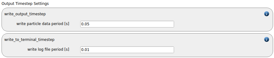
The “output_settings” command the takes care that all particle information and the meshes are written to files accordingly. Furthermore it triggers the output of global quantities such as the kinetic energy of the particles or total normal and shear stresses onto meshes in the terminal.

We keep the default output_settings command:

Remark: please note that per default all meshes are written by the output settings, but without potentially available values for stress, wear, velocity etc. Please use the mesh_properties command for producing the desired output. If meshes are added to the meshes list but no mesh_properties are selected, all available properties will be written by default.

The setup of this case is complete now, we can save the setup and move on to the simulate section.

Running the case

The simulation should be simulated on two cores, therefore we change the number of processors to two:

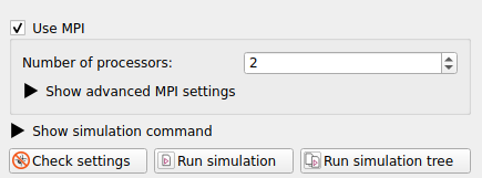
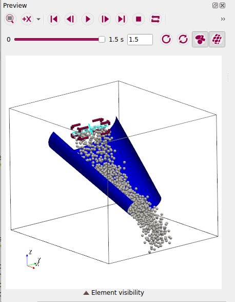
Next one can either run check the simulation setup (“Check settings”) or start with the simulation run (“Run simulation”) right away. While the simulation is running, the particles can already be previewed in the graphics preview window:

Global simulation output is shown in the Line Charts section, here we visualized the number of particles, kinetic energy and force in z-direction onto the chute:

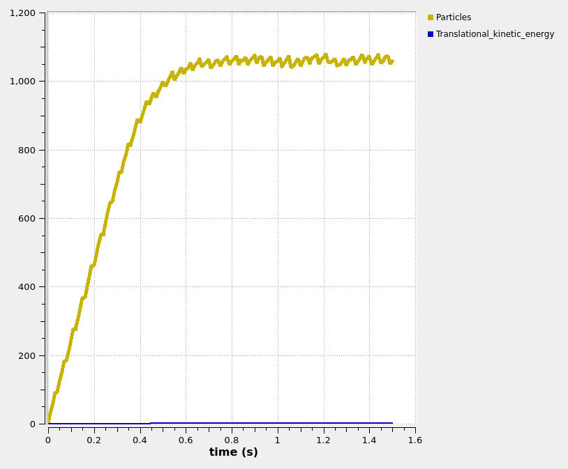
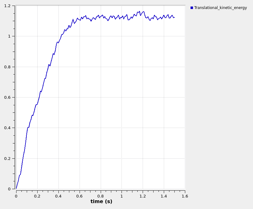
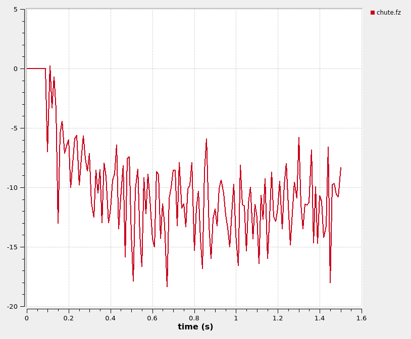
The data displayed in the graph can be edited and saved as image for further usage in reports and presentations.

Postprocessing

As soon as data was written to the post-folder within the simulation, it can be displayed with Paraview or Ovito.

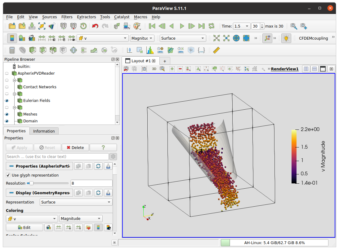
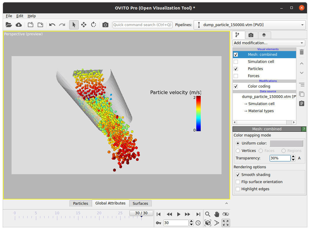
Both software packages provide numerous tools and filters for an optimal visualization of the results.