Multisphere Mixer

In this test case a more complex geometry is used: several meshes are loaded and positioned accordingly. In a first simulation, multispheres are inserted in four different regions, while the geomtry is at rest. In a second simulation the geometry starts moving and thus mixes the previously inserted multisphere particles.

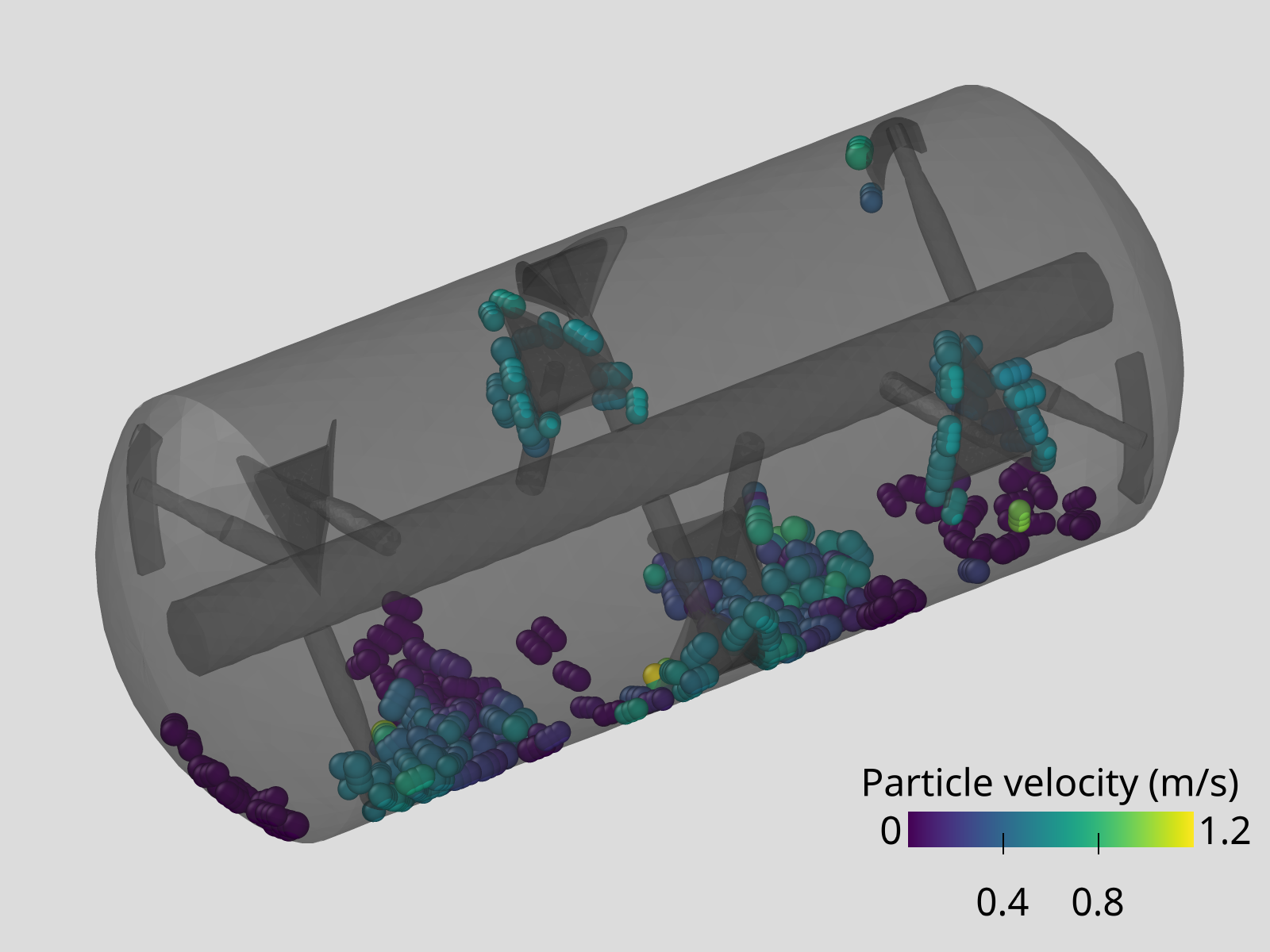
Discussed features are the generation and insertion of multisphere particles and the mesh motion.

Name of the case: Project_Mixer_Multispheres

Inserting multispheres into a Mixing Drum

General settings

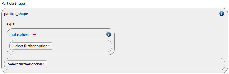
In this simulation we use particles of particle_shape command multisphere:

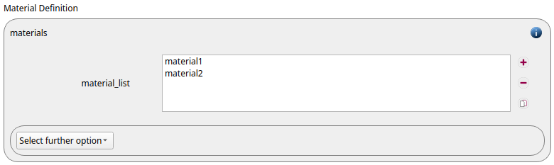
Two materials command, material1 and material2, are defined:

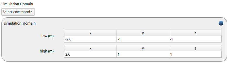
The simulation domain is defined with x dimension ranging from -2.6 to 2.6 meters and y and z dimensions ranging from -1 to 1 meters:

Meshes and regions

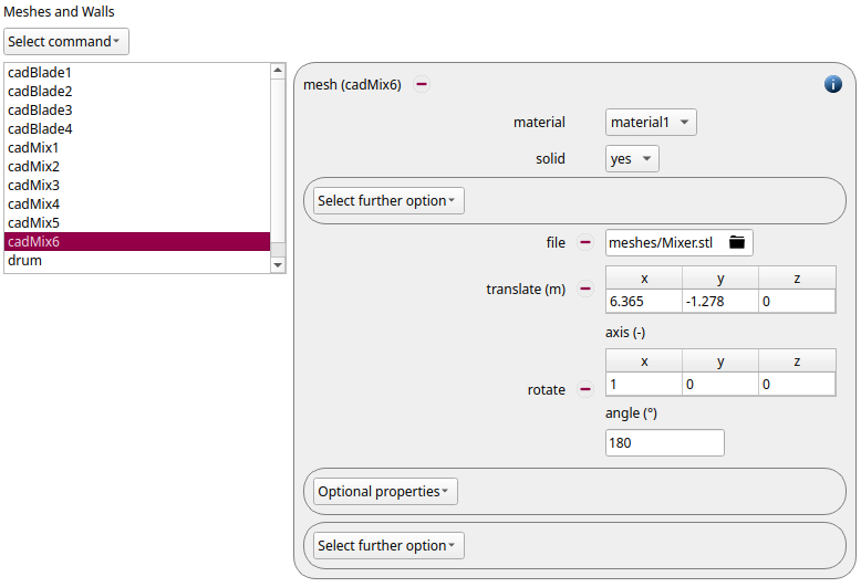
As mentioned in the introduction a rather complex geometry is used in that case. We start with inserting the shaft and the four blades, using the mesh command command. All these five components are of material1 and need to be translated by (4.175, -1.278, 0):

Since they will be used as walls, make sure that the option solid is set to yes (default).

The insertion of the mixer paddels is slightly more complex, as we use the same stl-file (Mixer.stl) but translate and rotate it differently:

	translate	rotation axis	angle of rotation (in deg)
cadMix1	(4.175 -1.278 0)	(- - -)	(- - -)
cadMix2	(4.7225 -1.278 0)	(1 0 0)	240
cadMix3	(5.27 -1.278 0)	(1 0 0)	300
cadMix4	(5.27 -1.278 0)	(1 0 0)	120
cadMix5	(5.8174 -1.278 0)	(1 0 0)	60
cadMix6	(6.365 -1.278 0)	(1 0 0)	180

Finally a drum is inserted. This mesh needs to be scaled by the factor 1.001. The complete list of meshes contains 12 elements:

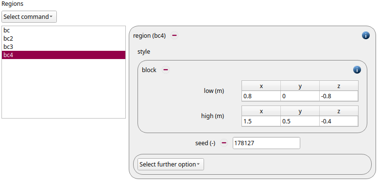
The particles are generated in four regions of shape block with the following dimensions:

	xmin	xmax	ymin	ymax	zmin	zmax
bc	-1.1	-0.4	-0.5	0.0	-0.8	-0.4
bc2	0.8	1.5	-0.5	0.0	-0.8	-0.4
bc3	-1.1	-0.4	0.0	0.5	-0.8	-0.4
bc4	0.8	1.5	0.0	0.5	-0.8	-0.4

Physics models

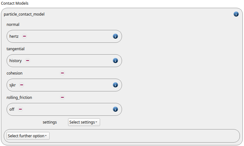
In the next step, the definition of the physics models takes place. For the particles we use the normal contact model hertz and the tangential model history. For cohesion the sjkr model is used:

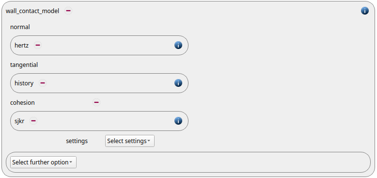
Since we added meshes in the previous section, also a wall contact model was added automatically in this section. We use the same contact models as for the particles:

Finally also the gravity is defined:

Per default the gravity has a magnitude of 9.807 and acts into negative z-direction. These defaults can be changed by either setting the magnitude or the direction manually.

Particles

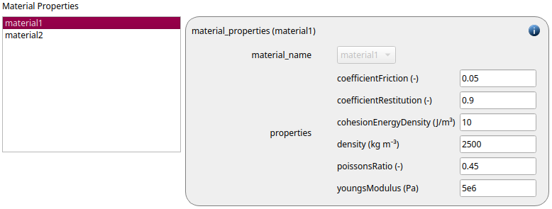
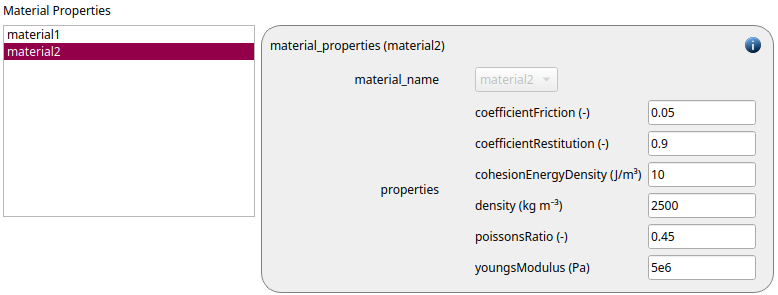
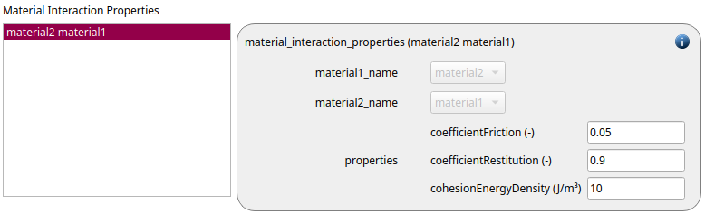
In the general settings tab we introduced two materials. Here we define the required material properties and material interaction properties.

	material1	material2
Density	2500	2500
Young’s modulus	5e6	5e6
Poisson ratio	0.45	0.45
Coefficient of restitution	0.9	0.9
Coefficient of friction	0.05	0.05
Cohesion energy density	10	10

	material1 / material2
Coefficient of restitution	0.9
Coefficient of friction	0.05
Cohesion energy density	10

In the next step the particle templates are generated. As multispheres should be used, one first opens the multisphere builder under tools/MS Builder. This tool allows the user to build arbitraty multispheres defining the number of spheres, the center position of each sphere and its radius:

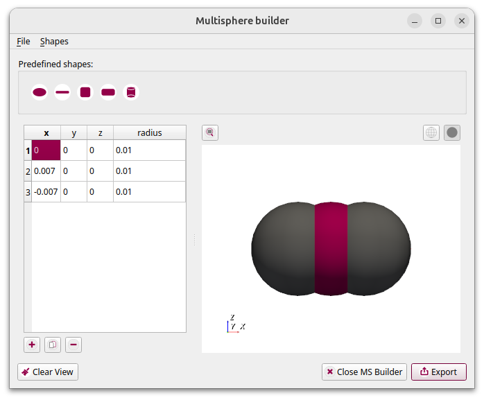
The multispheres are visualized. Depending on the size you might need to zoom in. In this case three multispheres are created, each of them consists of three spheres:

Multisphere 1:

	x	y	z	radius
sphere 1	0.0	0.0	0.0	0.01
sphere 2	0.007	0.0	0.0	0.01
sphere 3	-0.007	0.0	0.0	0.01

Multisphere 2:

	x	y	z	radius
sphere 1	-0.0065	0.0	0.0	0.009
sphere 2	0.0	0.0	0.0	0.009
sphere 3	0.0065	0.0	0.0	0.009

Multisphere 3:

	x	y	z	radius
sphere 1	-0.0075	0.0	0.0	0.011
sphere 2	0.0	0.0	0.0	0.011
sphere 3	0.0075	0.0	0.0	0.011

Please save the multispheres in separate csv files (e.g. p_0_01.csv, p_0_009.csv, p_0_011.csv), ideally in a “data” folder within the current simulation.

In the next step particle templates of shape multisphere are generated. Altogether six types with the following settings are defined:

	material	file (multisphere)	scale
p1	material1	p_0_01.csv	5
p2	material1	p_0_009.csv	5
p3	material1	p_0_011.csv	5
p4	material2	p_0_01.csv	5
p5	material2	p_0_009.csv	5
p6	material2	p_0_011.csv	5

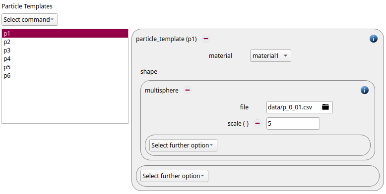
These six particle templates are used to define two particle distributions, one for each material type:

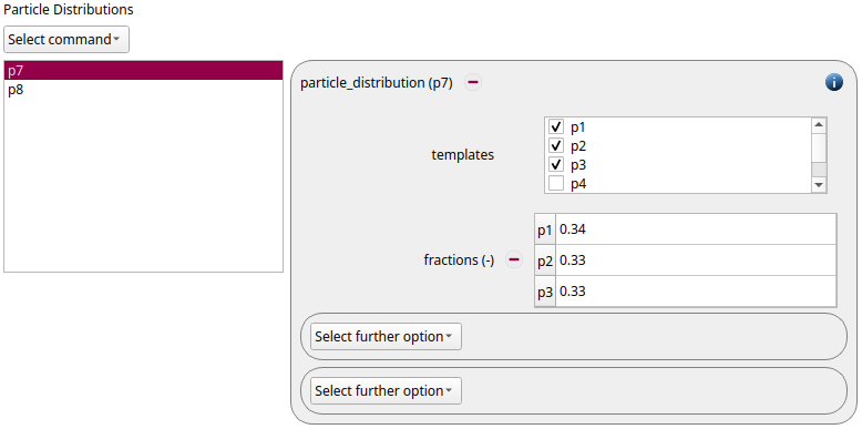
The first distribution consists of 34% particles of type p1, and 33% of type p2 and p3, the second distribution consists of 34% particles of type p4, and 33% of type p5 and p6.

These distributions are now inserted in the four previously defined insertion regions. We use four insertion command commands with mode pack. In region bc and bc2 particles with the first distribution are used, in regions bc3 and b4 particles with the second distribution are inserted. These are the settings for the insertion:

	region	insert_every_time	target_mass	particle_distribution	velocity
i1	bc	3e-2	50	p7	constant (0 0 -0.5)
i2	bc2	3e-2	50	p7	constant (0 0 -0.5)
i3	bc3	3e-2	50	p8	constant (0 0 -0.5)
i4	bc4	3e-2	50	p8	constant (0 0 -0.5)

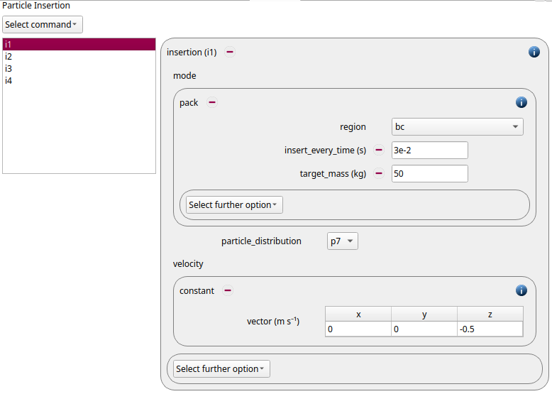
Simulation control

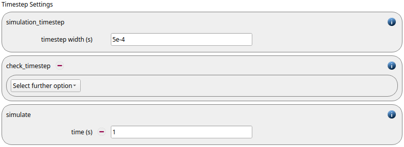
In this tab one first choses the time step settings such as the desired simulation timestep of 1e-5 seconds and the total simulation time of 1.0 second. Per default also the check_timestep command command is enabled, which throws a warning when the time step exceeds 10 % of the Rayleigh or the Hertz timestep. These thresholds can be changed by setting an alternative value for hertz_fraction or rayleigh_fraction.

Output settings

In this tab we first define the timestep width for the file and the terminal output:

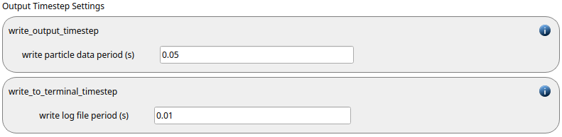
The output_settings command command takes care that all particle information and the meshes are written to files accordingly. Furthermore it triggers the output of global quantities such as the kinetic energy of the particles or total normal and shear stresses onto meshes in the terminal. Please note that if the output of per-cell information on meshes such as wear, velocity or stress are desired, the keyword mesh_properties has to be added and the required output has to be selected.

Running the simulation

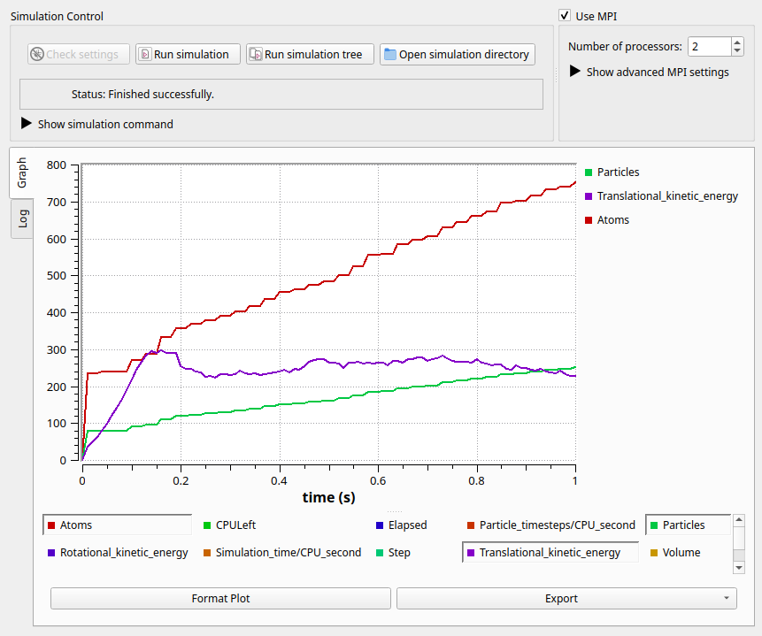
After saving the case we can change to the Simulation section. By hitting the Start button we can start running the simulation either serially or in parallel, using mpi:

Result

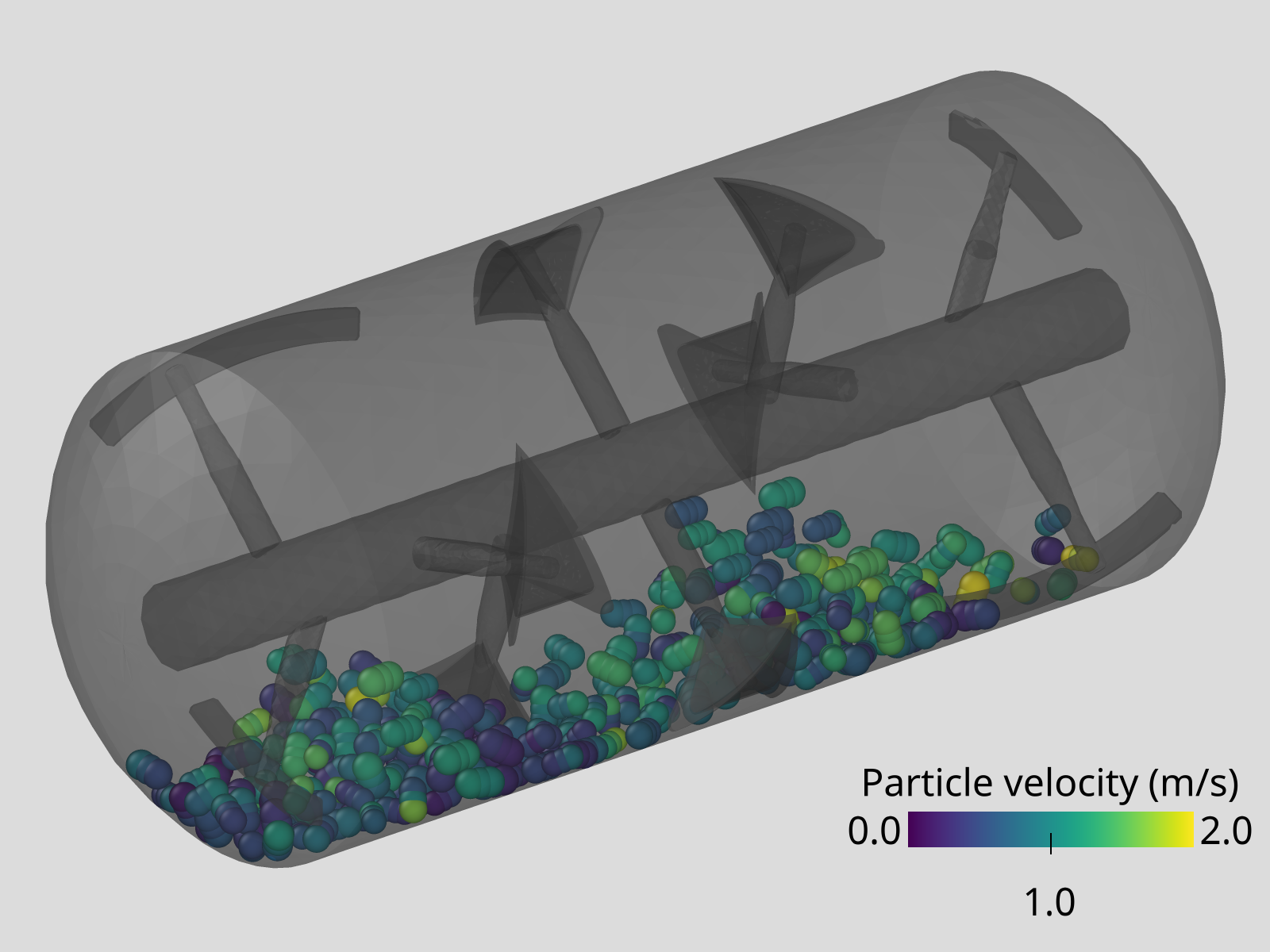
The result of the calculation can then be visualized with Paraview:

Mixing by mesh motion

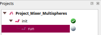
The existing simulation can be continued by hitting the Derive simulation button underneath the orginal simulation. This leads to a freeze of the original simulation (i.e. no further changes of the setup are permitted) and the generation of a second simulation, which shares most of the settings with the original simulation. The main difference lies in the fact that the new simulation will be started with the data produced in the last time step of the parent simulation. After renaming the new simulation the time-line looks as follows:

A derived simulation always uses the same particle shape, simulation domain (both by means of dimensions and boundary style) and materials as the parent simulation, thus all the quantities in the General Settings tab are locked.

Meshes

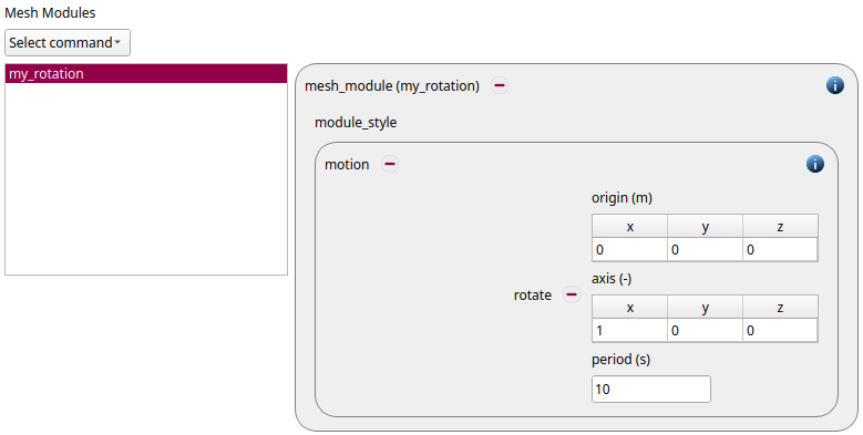
The motion of the meshes is induced by a mesh module of type motion:

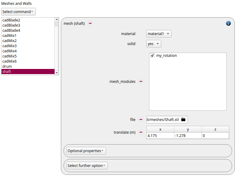
This module has to be activated for all meshes except for the drum:

Particles

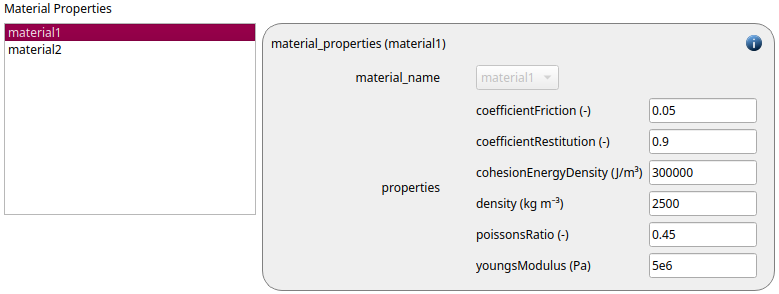
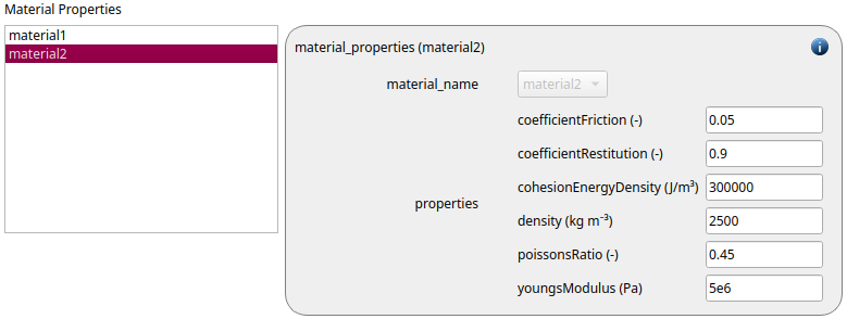
The particle properties remain the same apart from the cohesion energy density for the cohesion model sjkr. We change it to 300000 for both materials:

As the desired amount of particles has already been inserted in the original simulation, the insertion commands can be removed. After doing so one can proceed with removing the particle distributions and the templates. Due to dependencies it is important to keep that order.

Regions

Just as the meshes before also the insertion regions were preserved. As no insertion will take place (and there remain no dependencies due to the removal of the insertion commands in the previous step) the regions can be removed as well.

Simulation control

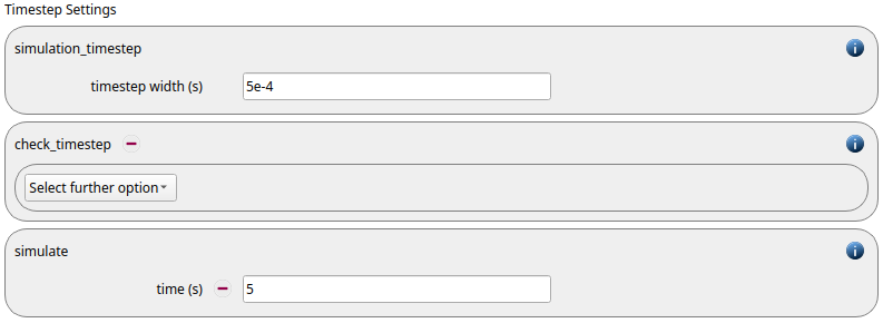
As a period of 10 was selected for the mesh rotation, the simulation time should be increased, in this case it is changed to 5 seconds. The rest of the settings remain the same.

Please note that due to the complexity of the case (particularly the rotation of the meshes) this simulation will take some time.

Output settings

We add two calculate command commands for determining the center of mass and the mixing index:

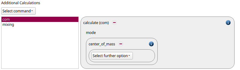
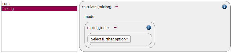
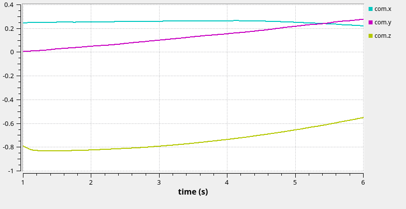
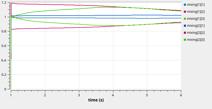
The center of mass and mixing index lead to the output of text-files. The output files for the mixing index are named according to the order of the material definitions in the general settings tab. The mixing index is of interest if particle templates with different materials are used. Materials that are only used for walls have a mixing index of 0. The files will be written to the simulation folder during the calculation and can for example be postprocessed with Matlab, Octave or Excel. The global output is also written to the line plot during the simulation, the quantities are referenced by their IDs (com and mixing).

Result

As soon as all settings are completed the calculation we set the number of MPI processes to two and run the simulation.

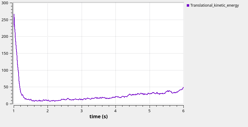
This graph shows the kinetic energy of the system thoughout the calculation:

Also, the center of mass and the mixing index can be visualized:

The result can again be visualized with Paraview: