Electrical conductivity

The main topic of this tutorial is electrical conductivity. In a first simulation we create a packing of soft particles with large overlaps and thus contact areas (achieved by compressing the particles). In the second step, heat conduction and electrical conductivity (with electrical heating) are switched on. The particle-particle and particle-wall contact network can be added to the output such that electric current and electric conductance can be visualized.

Name of the case: Project_Electrical_Conductivity

Case 1: Insertion

First, the used materials command as well as the simulation domain are defined in the General Settings tab. Please note that the dimensions of the simulation domain can only be defined in the first simulation. This means that the box that forms the simulation domain has to be chosen big enough from the beginning.

General settings

In this simulation we set particles of particle shape sphere:

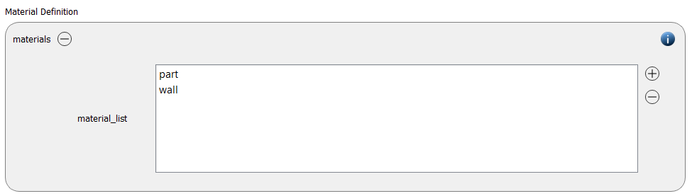
A single materials command with the name default is used:

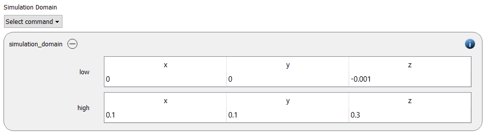
The simulation domain is defined with x and y dimensions ranging from 0 to 0.1 meters, and z domain ranging from -0.001 to 0.3 meters.

Meshes and regions

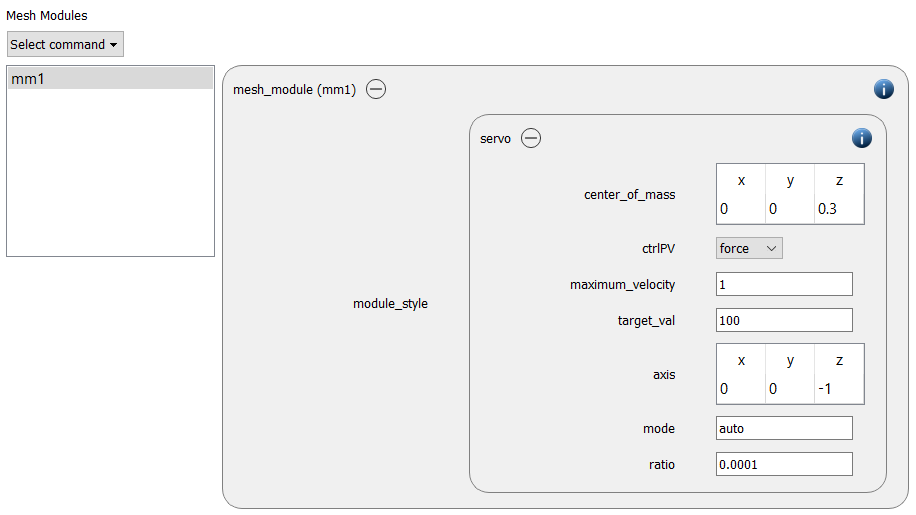
First, we create a mesh module the converts the top wall into a servo wall that compresses the particles:

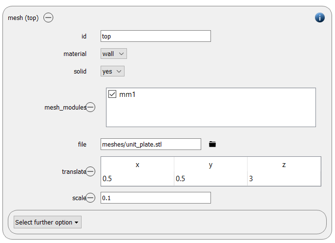
The mesh command command is then used to load the top plate geometry and the mesh module “mm1” is activated:

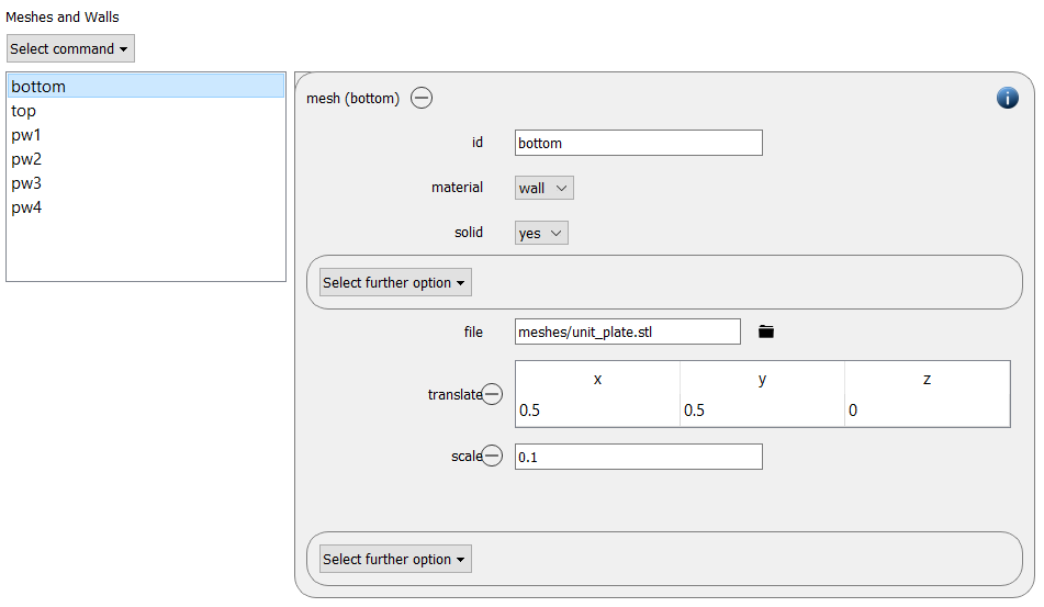
Another mesh command is used to insert a bottom plate:

Four primitive walls of type plane are used as x any y walls with an offset of 0 and 0.1:

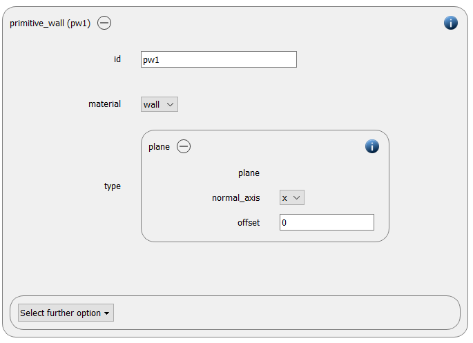
Physics models

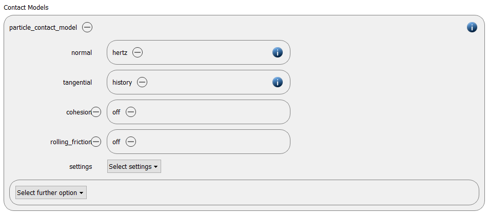
In the next step, the definition of the physics models takes place. For the particles we use the normal contact model hertz and the tangential model history.

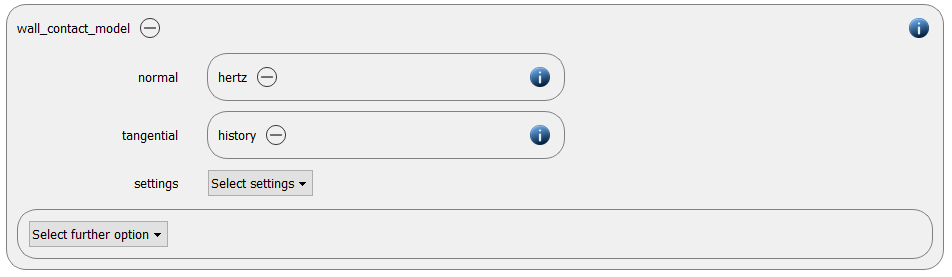
Since a wall mesh (the chute) was added in the previous section, a wall contact model is added automatically in this section. We use the same properties of the particle contact model:

Finally, the gravity command is removed from the setup.

Particles

In the general settings tab we defined two material types (part and wall), whose material properties have to be specified here:

	part	wall
density	100	1000
Young’s modulus	1e6	1e7
Poisson’s ratio	0.5	0.5
Coefficient of restitution	0.1	0.5
Coefficient of friction	0.1	0.5

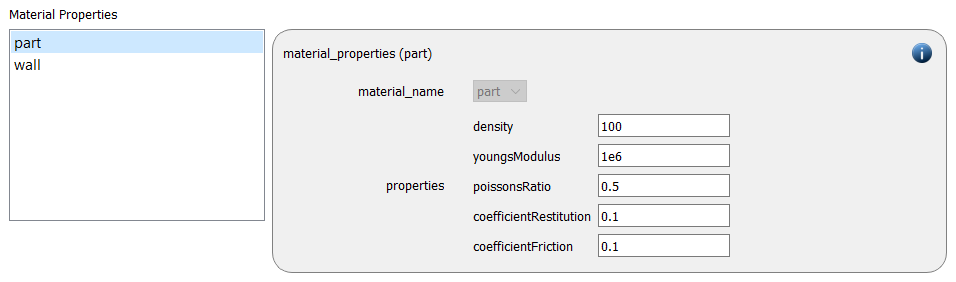
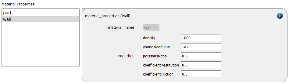
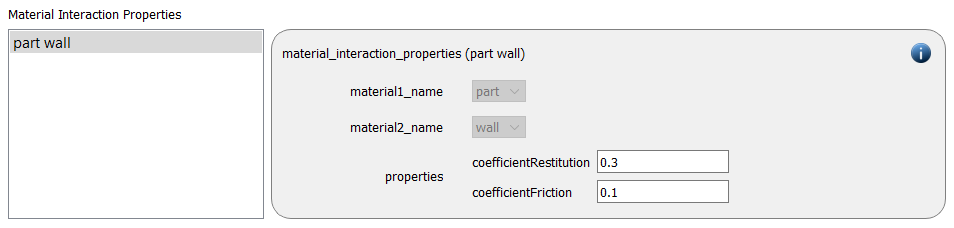
The material interaction properties are defined as following:

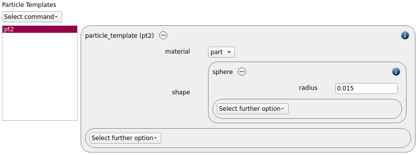
A template for spheres with radius of 0.015 meters is generated:

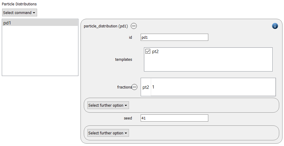
Based on this template a particle distribution is created:

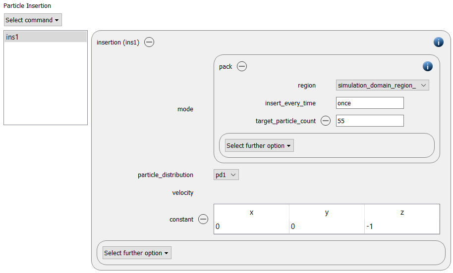
The final step in this tab is the definition of the insertion command. We add a pack of 55 particles once at the beginning of the simulation. The initial velocity of the particles is given with (0,0,-1) m/s.

Simulation control

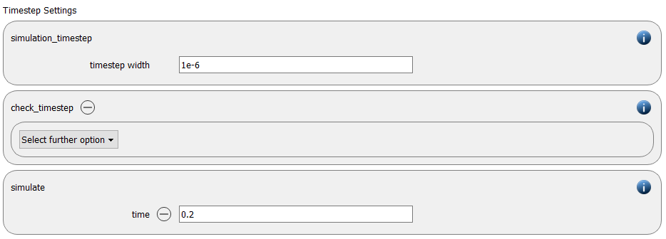
In this tab, one first choses the time step settings such as the desired simulation timestep of 1e-6 seconds and the total simulation time of 0.05 second. Per default, the check_timestep command command is also enabled, which throws a warning when the time step exceeds 10 % of the Rayleigh or the Hertz time. These thresholds can be changed by setting an alternative value for hertz_fraction or rayleigh_fraction.

Output settings

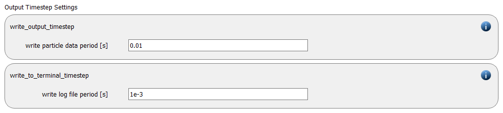
In this tab, we first define the timestep width for the file and the terminal output:

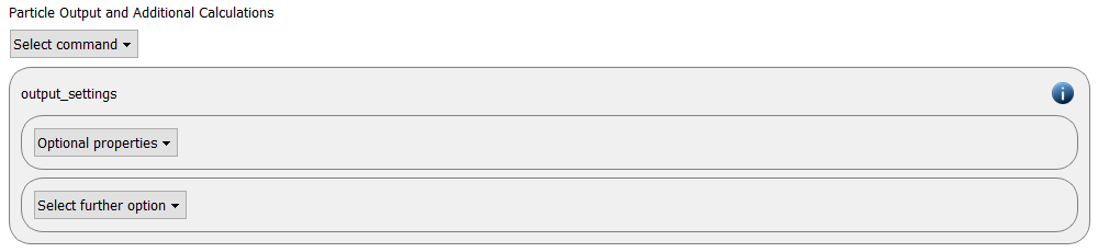
The output_settings command command takes care that all particle information and meshes are written to files. Furthermore, it triggers the output of global quantities such as the kinetic energy of the particles or total normal and shear stresses onto meshes to the terminal.

Custom commands

When using a Young’s modulus smaller then 5e6 Aspherix throws Warnings to inform the user that the particles are softer than usual for a DEM simulation. By adding the soft_particles command command we can suppress these warnings:

Simulation

After completing the setup and saving it, the simulation can be launched. Therefore, change to the Simulation view. First hit the “Check settings” button, and if the check returns “Check settings successfully completed” the simulation can be run by hitting “Start”:

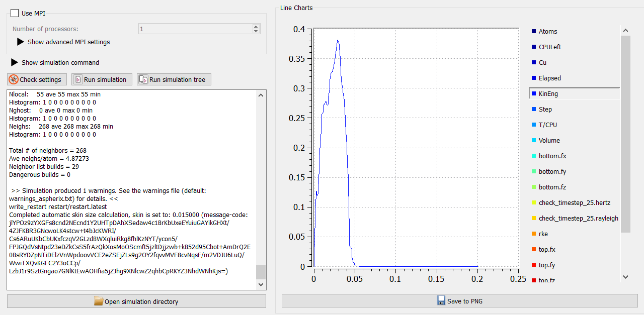
Since the setup only contains 200 particles, parallelization will not increase the simulation speed, the calculation can thus be carried out in serial.

Postprocessing

For postprocessing both Paraview and Ovito can be used.

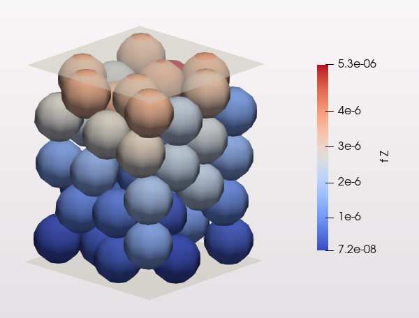
Particle bed in Paraview:

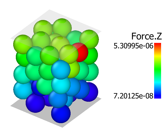
Particle bed in Ovito:

Case 2: Conductivity

In this second simulation we appyl heat transfer and electrical conductivity to the particle packing. The servo wall keeps the particles further in place.

Physics models

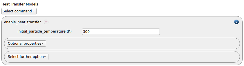
First, the heat transfer is enabled. The initial particle temperature is set to 300K.

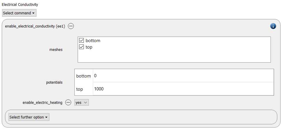
Then we add the enable_electrical_conductivity command command. The two meshes top and bottom are used, the potential of mesh “bottom” is set to 0 and the potential of the mesh “top” is set to 1000. Furthermore, electric heating is switched on:

Particles

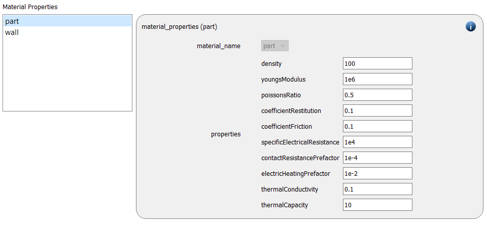
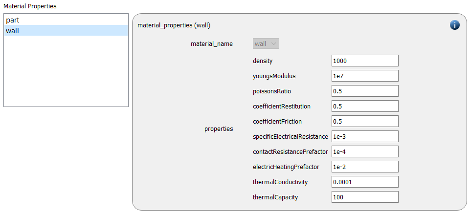
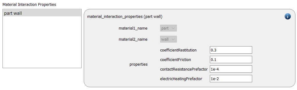
By adding the two previous commands, additional material properties and material interaction properties became necessary:

No further particles are meant to be inserted in this step, therefore the insertion command had to be removed:

Particle distribution as well as particle template can but do not have to be removed.

Simulation

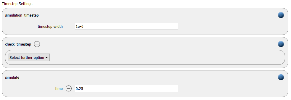
The simulation time is increased to 0.25 seconds:

Output

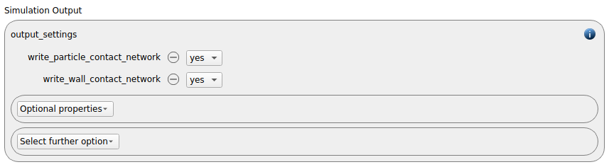
The contact network is calculated automatically. Please set “write_particle_contact_network” and “write_wall_contact_network” to yes and define the id of the wall contact network (id from previous command):

Simulation

Again, the simulation can be run on a single core. The plot shows the kinetic energy during the calculation:

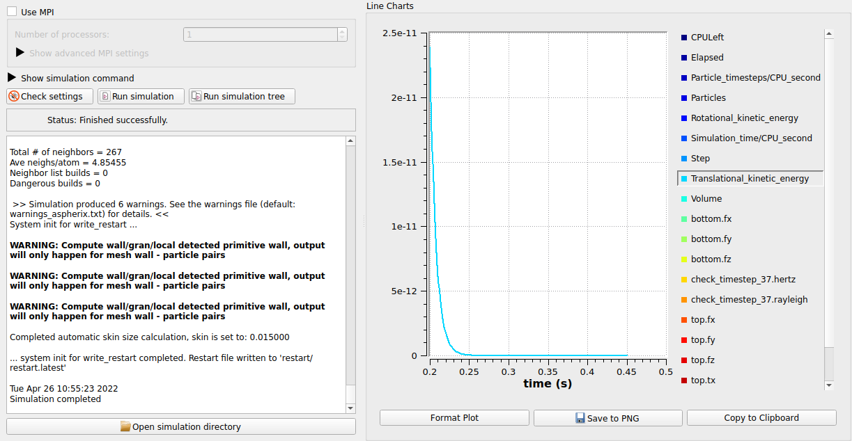
Remark: the displayed warnings indicate that particle-wall contacts can only be displayed between meshes and particles but not between primitive walls (side walls in our case) and particles, which is fine for our case setup.

Postprocessing

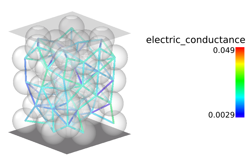
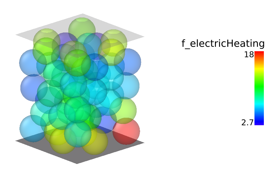
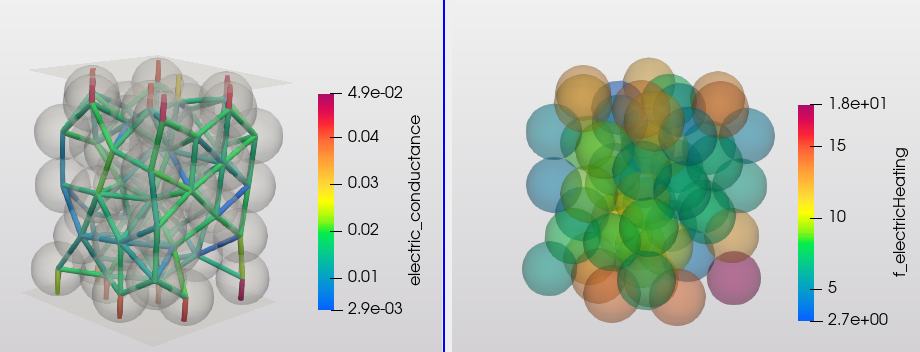
The results can be postprocessed both in Paraview and Ovito. The images below show the results at the last time step, coloring is according to electric conductance (contacts) and electric heating (particles).

Ovito supports the visualization of particle-particle contacts, particle-wall contacts can currently not be displayed:

---