Measure Potential

The main topic of this tutorial is the measurement of the electric potential within a bed with the help of meshes, as well as the usage of the simulation mode “simulate until_condition_reached”. In a first simulation we insert a pack of particles in a cylindric domain that contains two probe-tubes and let them settle initially. In the second step we apply a force to compress the particle bed, the simulation stops once the average stress on the compression wall reaches a steady state. Finally, in the last simulation, we enable electrical conductivity and apply a current at the bottom, that heats the particles in the bed. The potential can be evaluated both at the top mesh and both probe tubes. The simulation ends when the average temperature of the particle bed is converged.

Name of the case: Project_Measure_Potential

Case 1: Pre-Compaction

First, the used materials command as well as the simulation domain are defined in the General Settings tab. Please note that the dimensions of the simulation domain can only be defined in the first simulation. This means that the box that forms the simulation domain has to be chosen big enough from the beginning.

General settings

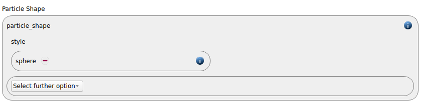
In this simulation we set particles of particle shape sphere:

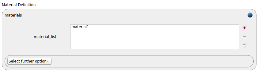
A single materials command with the name default is used:

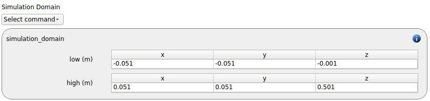
The simulation domain is defined with x and y dimensions ranging from -0.051 to 0.051 meters, and z domain ranging from -0.001 to 0.501 meters.

Meshes and Regions

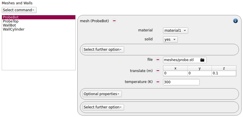
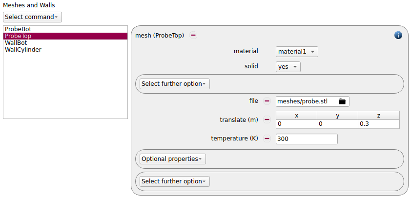
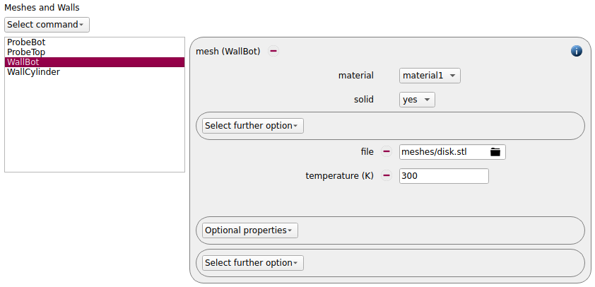
We add three meshes ProbeBot, ProbeTop and Wall, all of material material1, solid yes and temperature 300K:

	ProbeBot	ProbeTop	WallBot
file	probe.stl	probe.stl	disk.stl
translate	(0,0,0.1)	(0,0,0.1)	—

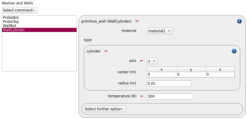
A cylindric primitive wall is used as side wall:

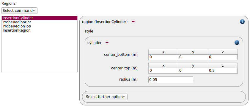
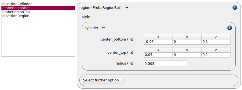
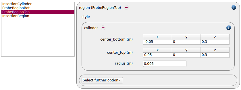
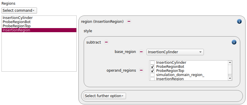
The insertion region consists of a vertical cylinder, from which the regions of the probes are subtracted to avoid overlaps during the insertion:

Physics models

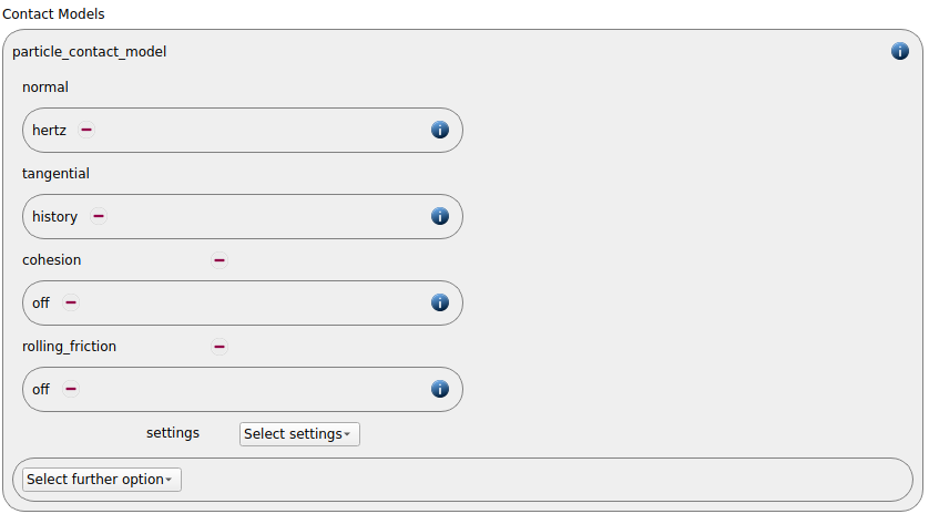
In the next step, the definition of the physics models takes place. For the particles we use the normal contact model hertz and the tangential model history.

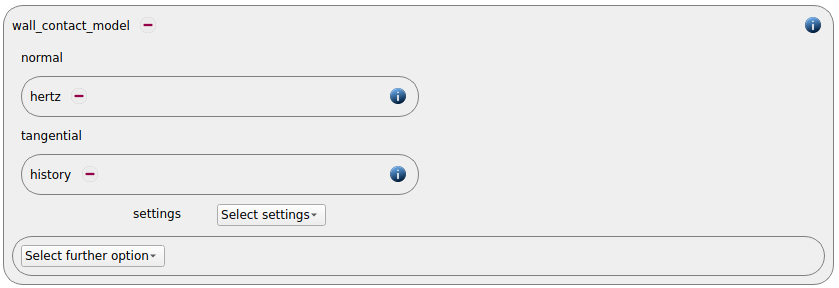
Since wall meshes were added in the previous section, a wall contact model is added automatically in this section. We use the same properties of the particle contact model:

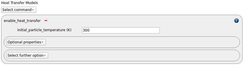
We add an enable_heat_transfer command command to track the heating of the particle bed later on:

Finally, also the gravity is defined:

Per default the gravity has a magnitude of 9.807 and acts into negative z-direction. These defaults can be changed by either setting the magnitude or the direction manually.

Particles

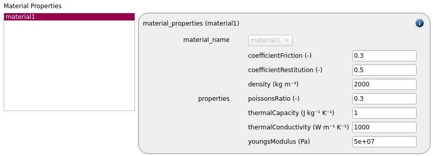
In the general settings tab we defined two material types (part and wall), whose material properties have to be specified here:

	material1
density	100
Young’s modulus	5e7
Poisson’s ratio	0.3
Coefficient of restitution	0.5
Coefficient of friction	0.3
Thermal Capacity	1
Thermal Conductivity	1000

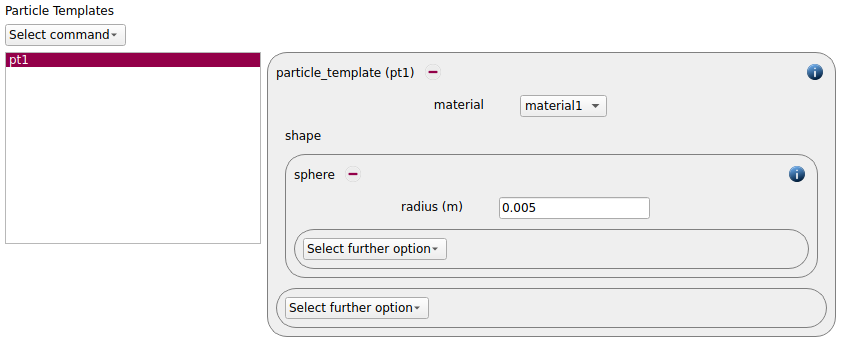
A template for spheres with radius of 0.005 meters is generated:

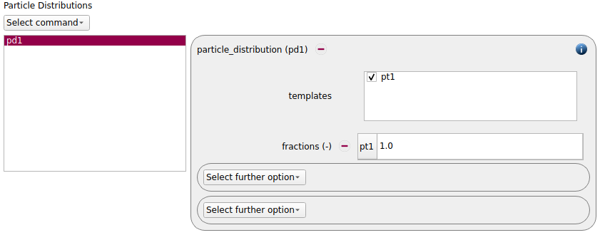
Based on this template a particle distribution is created:

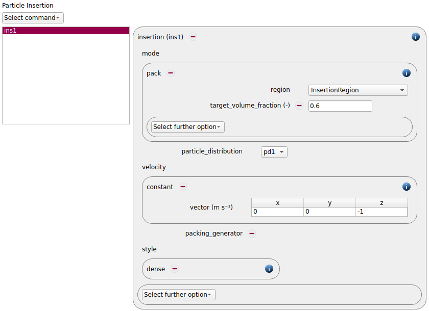
The final step in this tab is the definition of the insertion command. We add a pack of particles once at the beginning of the simulation, the target volume fraction is set to 0.6. We use the dense paricle generator dense. The initial velocity of the particles is given with (0,0,-1) m/s.

Simulation control

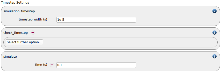
In this tab, one first choses the time step settings such as the desired simulation timestep of 1e-6 seconds and the total simulation time of 0.1 second. Per default, the check_timestep command command is also enabled, which throws a warning when the time step exceeds 10 % of the Rayleigh or the Hertz time. These thresholds can be changed by setting an alternative value for hertz_fraction or rayleigh_fraction.

For an optimal distribution of the loads on the processors we activate the loadbalancing:

Output settings

In this tab, we first define the timestep width for the file and the terminal output:

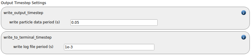
The output_settings command command takes care that all particle information and meshes are written to files. Furthermore, it triggers the output of global quantities such as the kinetic energy of the particles or total normal and shear stresses onto meshes to the terminal.

Simulation

After completing the setup and saving it, the simulation can be launched. Therefore, change to the Simulation view.

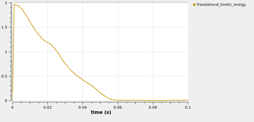
The image shows the kinetic energy:

Case 2: Create Packing

In this second simulation compress the particle bed with a servo wall.

Meshes and Regions

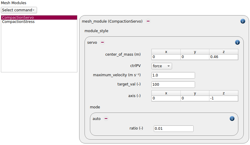
We therefore first add a mesh_module servo:

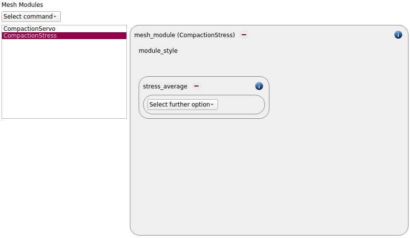
Then we add a mesh_module stress_average:

In the next step a mesh is added, to which both mesh modules are applied to:

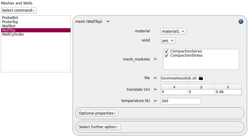
The upper position of the mesh as well as the center of mass of the servo wall is chosen based on the result of the initial simulation.

Since no more particles are required, we remove the insertion command in the Particles tab, and consequently we can also remove the insertion regions:

Simulation Control

We now want to run the simulation until the average stress on the top mesh reaches a steady state. We will do this by using the simulate command in mode until_condition_reached:

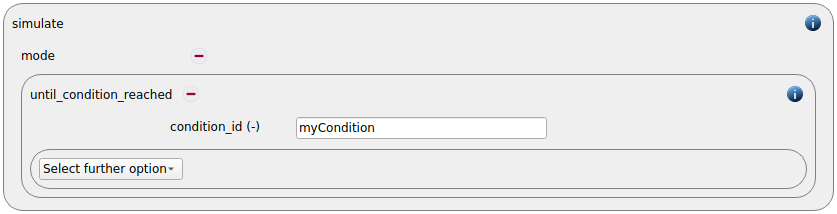
The condition myCondition will be defined later on.

Output Settings

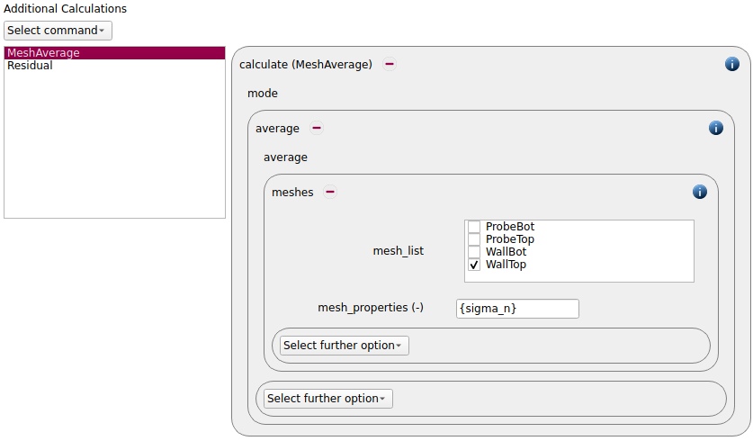
We add two new calculate commands, one to obtain the average stress on the mesh

and one to calculate the temporal residual of this quantity:

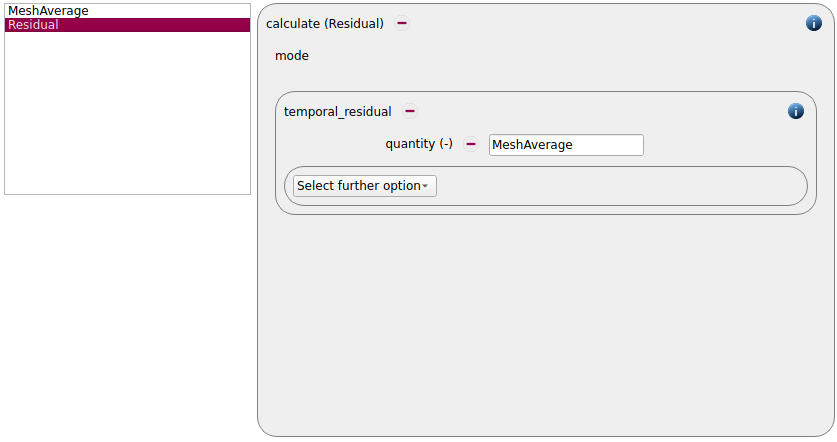
Custom Settings

Finally we define the boolean condition:

The weight 22 makes sure that the command is added before the simulate command (weight 25) that uses it.

Simulation

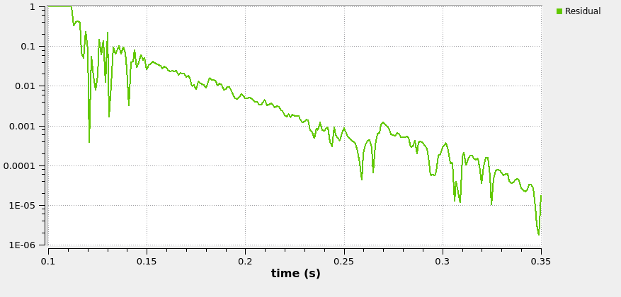
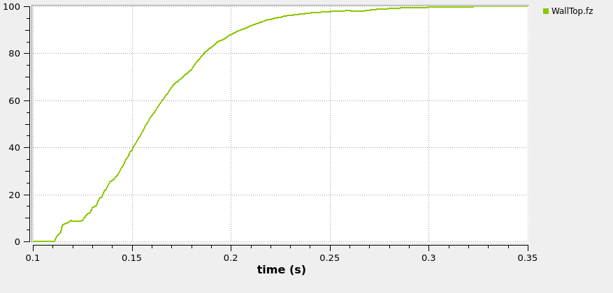
After the setup is completed, the simulation can be launched. The images below show the residual (logarithmic y-axis, use format plot for this) and the z-force onto the top wall:

Case 3: Electric Heating

In this last simulation we add the electric conductivity and simulate until the particle bed reaches a steady temperature.

Meshes and Regions

The mesh_modules keyword of the top wall is removed:

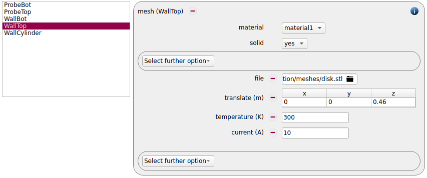
Both mesh_modules can be deleted as well.

At the top wall a current of 10 Ampere is applied. At the bottom wall we defined a potential of 0 Volt.

Physics Models

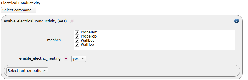
The enable_electrical_conductivity command is added and applied to all meshes in the simulation. The keyword enable_electric_heating is activated:

Particles

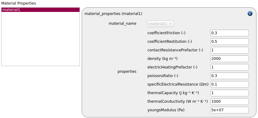
The material properties for the electrical conductivity and the heating have to be defined:

Simulation Control

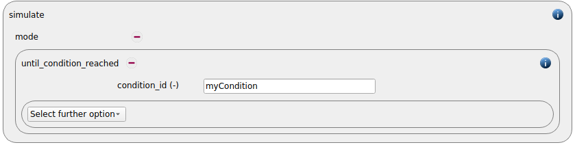
We keep the simulate command as is, but we will later on modify the condition to account for the average particle temperature instead:

Output Settings

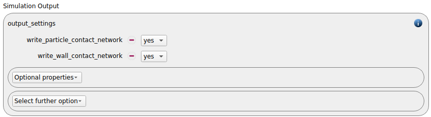
We add the keywords write_particle_contact_network and write_wall_contact_network to the output_settings command:

The previous calculate commands are replaced by a command that calculates the average particle temperature and its temporal residual:

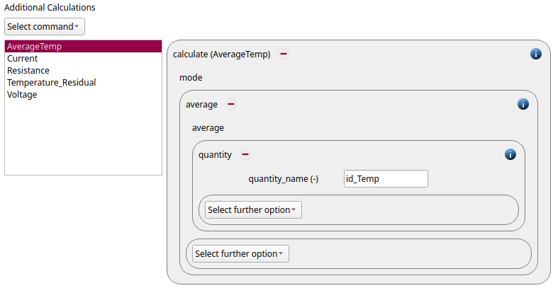
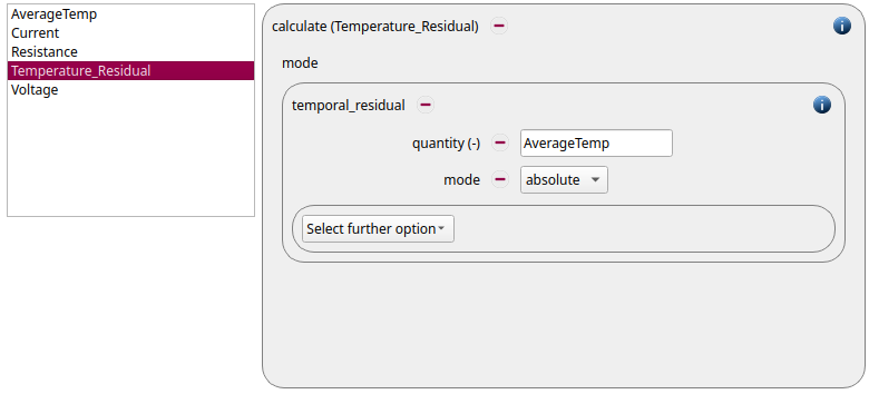
This time we use the absolute residual instead of the relative one, which is the default.

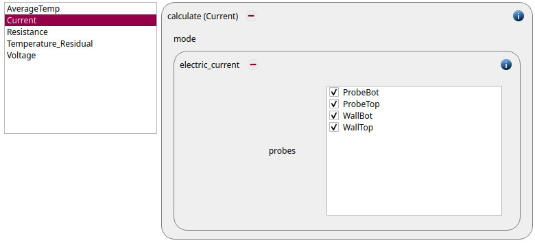
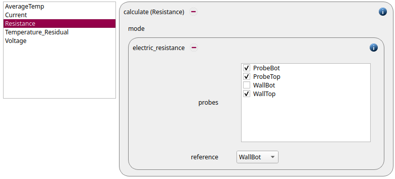
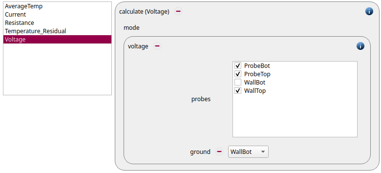
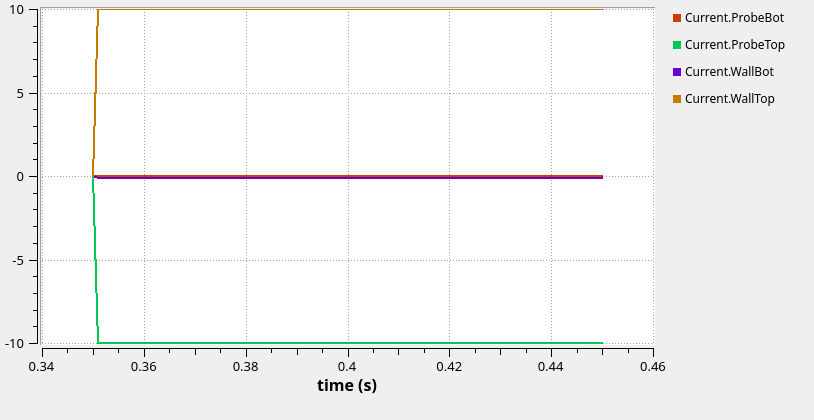
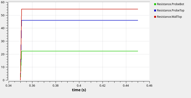
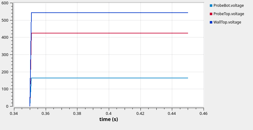
Furthermore, current, resistance and voltage between the bottom and top as well as the probes are calculated:

Custom Settings

Next, we modify the condition:

Expert Settings

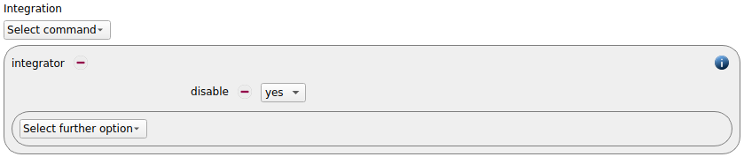
For speeding up the case we can now also disable the integrator:

Postprocessing

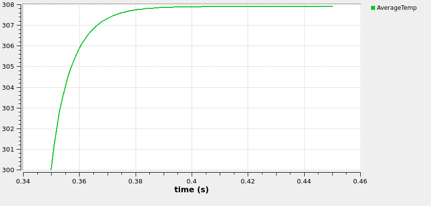
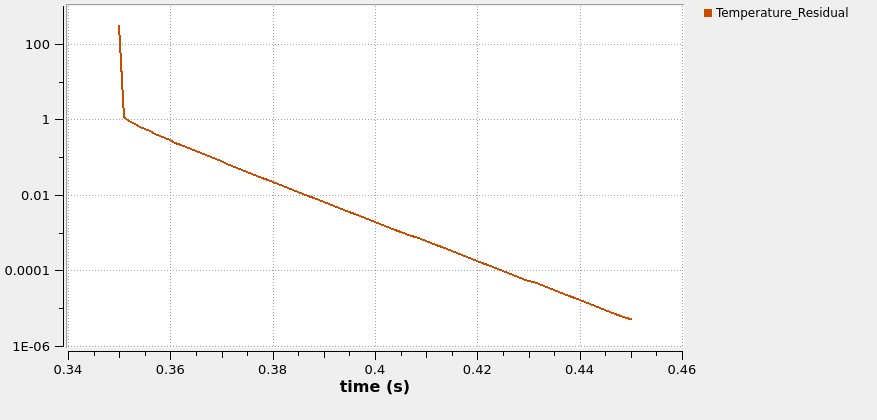
These graphs show the average particle temperature as well as the residual:

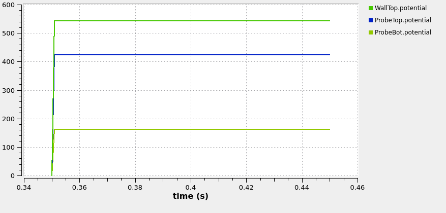
This image shows the potential at the two probes inside the mesh was well as at the top wall:

These graphs show electrical current, resistance and voltage:

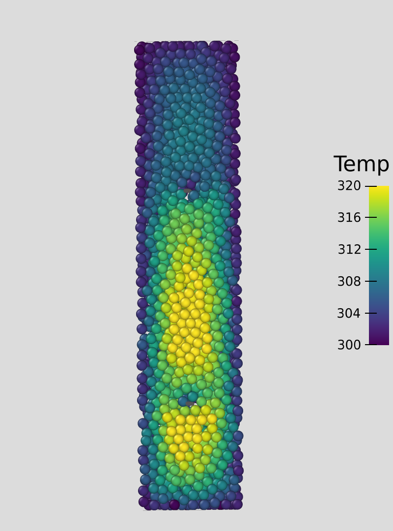
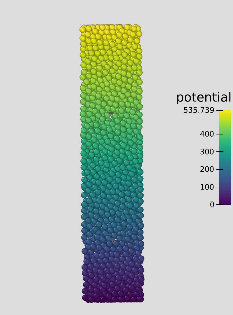
The results can also be visualized in Ovito or Paraview. These images show the particle bed colored according to temperature and electric potential at the end of the simulation:^

---