Conveyor with magnetic field for particle sorting

In this tutorial we insert a stream of particles into a conveyor, which are a mix of plastic and metal. The conveyor passes under a magnetic plate, whose magnetic field captures the metal particles and separate them from the plastic ones.

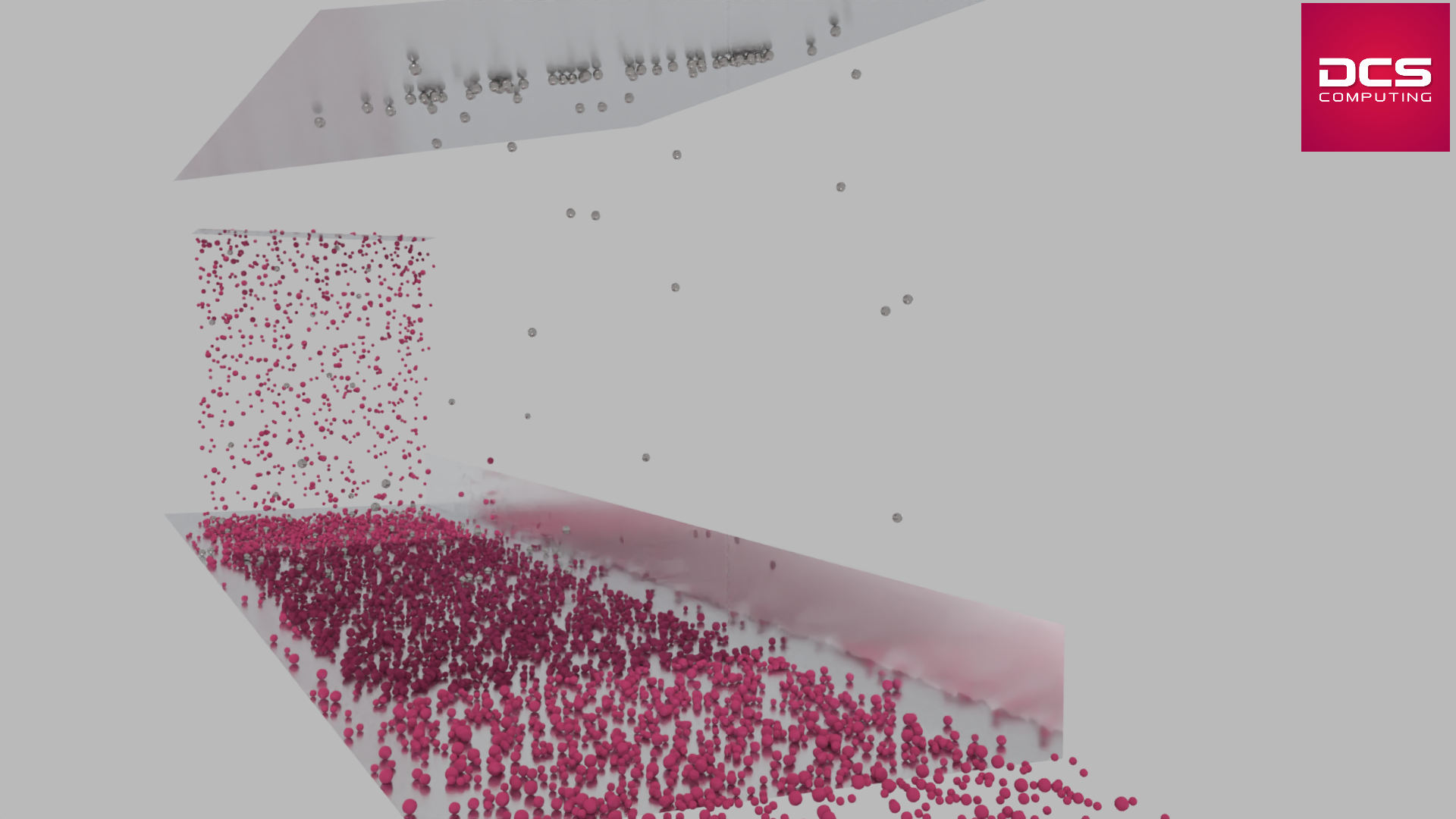
Name of the case: Project_Magnetic_Separation_Conveyor

Setting up the simulation

The first step is to define the particle shape, the used materials command and the simulation domain in the General Settings tab. Please note that in the case of multiple dependent simulations, the dimensions of the simulation domain can only be defined in the first simulation. This means that the box forming the simulation domain has to be chosen large enough from the beginning.

General settings

In this simulation we set particles of particle shape sphere:

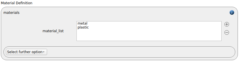
Two materials command are used, metal and plastic:

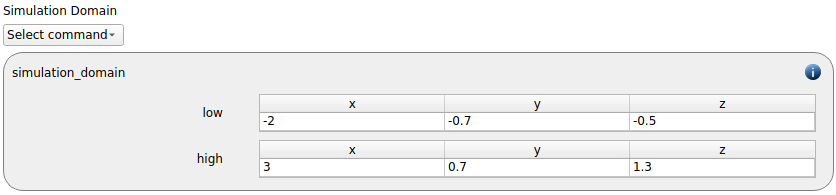
The simulation domain is set with the following dimensions:

	low	high
x	-2	3
y	-0.7	0.7
z	-0.5	1.3

Meshes and regions

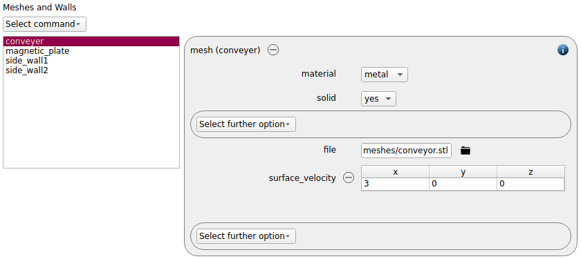
Five meshes need to be imported for this simulation: the conveyor and its two sidewall and the magnetic plate, all of which we insert via the mesh command command:

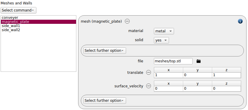
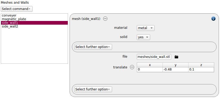
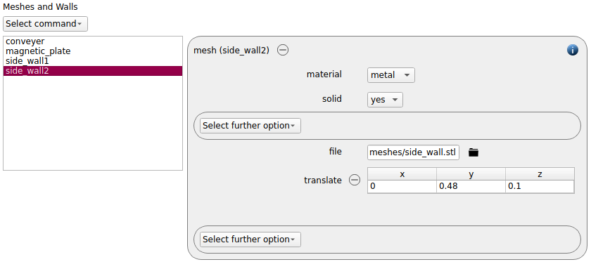
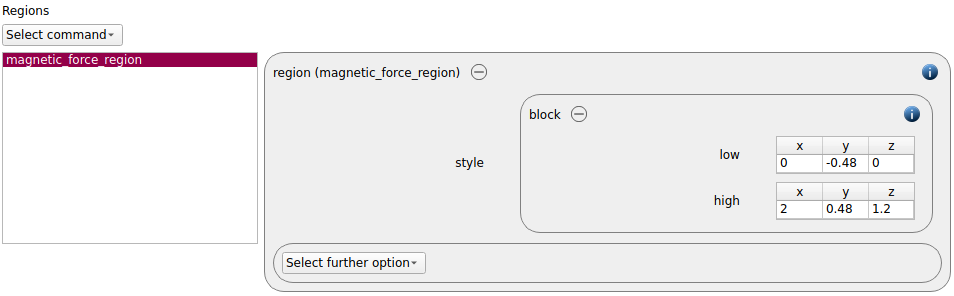
Here we also define the region where the magnetic field will act. We set the region with the following dimensions:

	low	high
x	0	2
y	-0.48	-0.48
z	0	1.2

Physics models

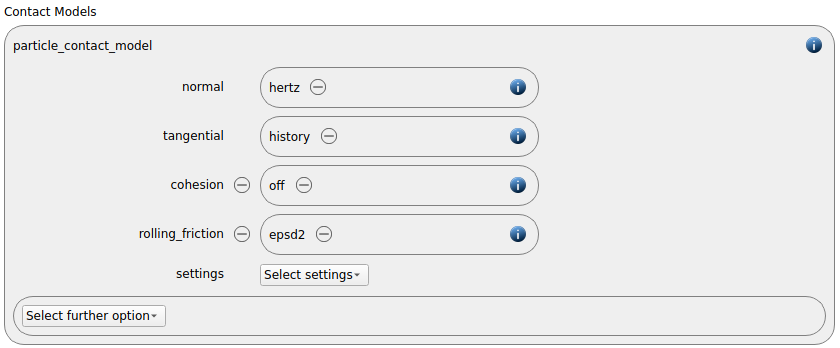
The contact models are defined now. For the particles we use the normal contact model hertz and the tangential model history, and the epsd2 model for rolling friction:

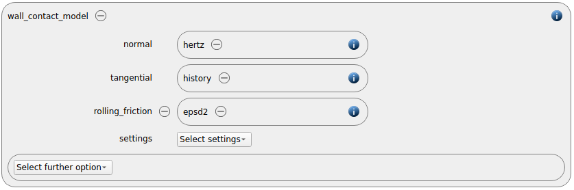
Since we added meshes in the previous section, a wall contact model is also added automatically to this section. We use the same properties as for the particle contact model:

Finally, gravity is enabled:

Per default gravity has a magnitude of 9.807 and acts into negative z-direction. These defaults can be changed by either setting the magnitude or the direction manually by hitting the “Select further option” button.

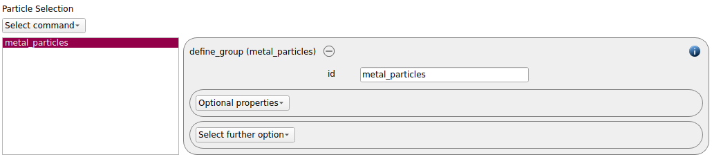
In this tab we must also define the magnetic force acting in the region we defined previously. This is done in the Body Force Models section (where enable_gravity is set), with the addforce/magnetic option. We set one magnetic field that is only visible for the metal particles. In order to allow for this restriction, we must first go to the Particles tab and add a define_group command command (Particle Selection section):

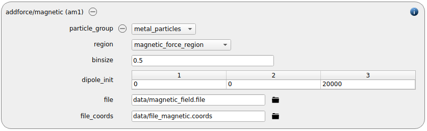
This particle group is the used in the definition of the particle template for the metal particles (see next step) and now also for the definition of the magetic force:

Particles

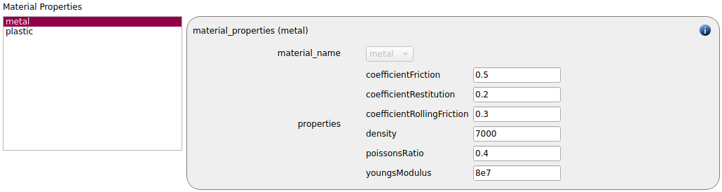
In the general settings tab we defined two material types, metal and plastic. The settings for both have to be specified here. The parameters for metal are:

	default
Density	7000
Young’s modulus	8e7
Poisson’s ratio	0.4
Coefficient of restitution	0.2
Coefficient of friction	0.5
Coefficient of rolling friction	0.3

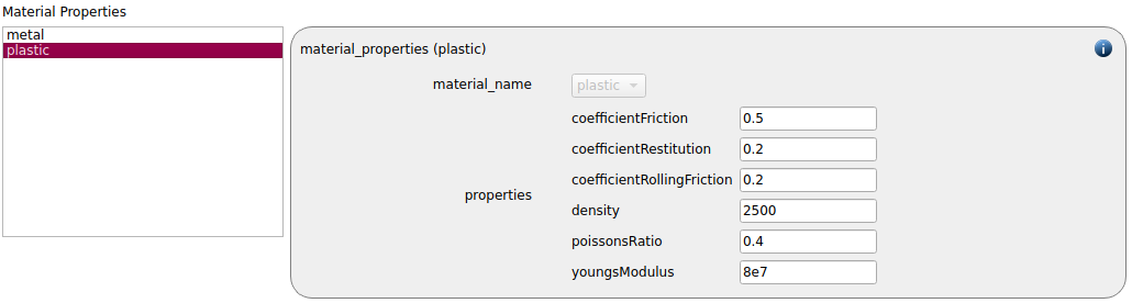
The parameters for plastic are:

	default
Density	2500
Young’s modulus	8e7
Poisson’s ratio	0.4
Coefficient of restitution	0.2
Coefficient of friction	0.5
Coefficient of rolling friction	0.2

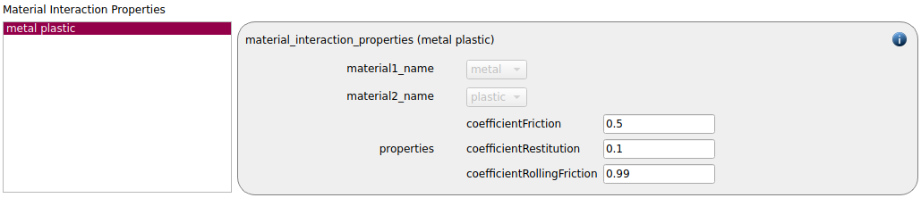
The material interaction properties are also defined:

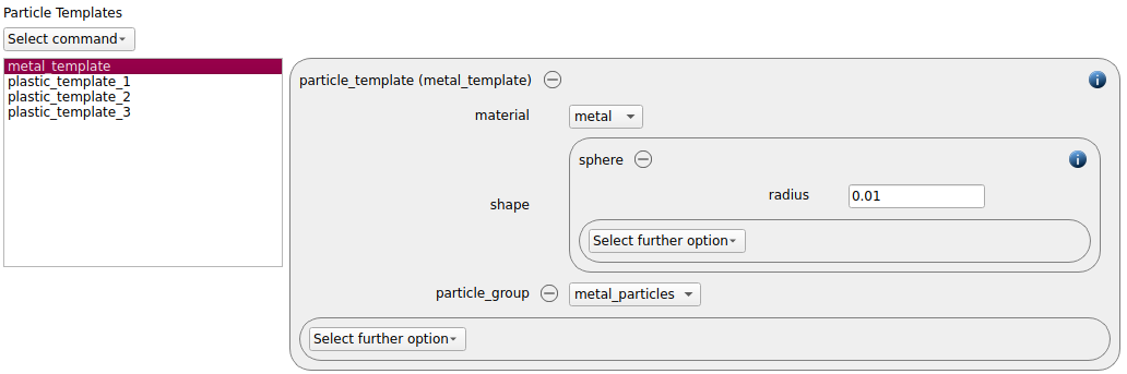
We now define four particle templates of shape sphere. Three of them are for plastic particles with different radii, one is for the metal particles. Note the group setting for each template. The groups are defined in the Expert Settings tab:

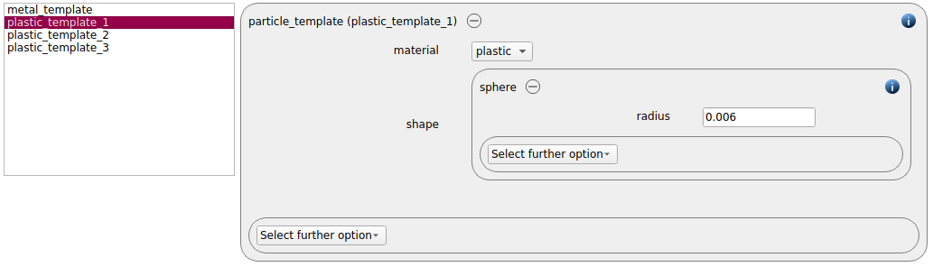
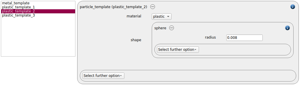
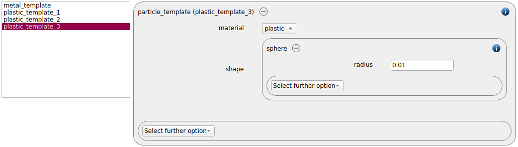
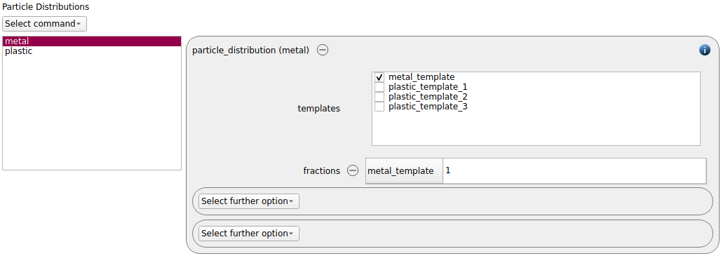
From these templates we make two particle distributions. One for the metal particles:

… and another one for the plastic particles, with fractions for each plastic particle template defined above:

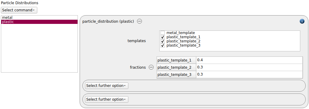
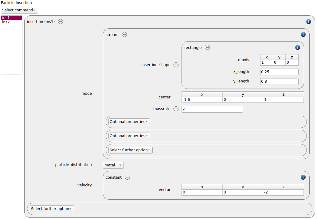
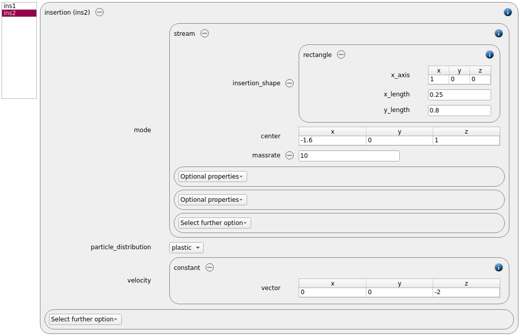
Each distribution will be used in its own insertion command command. Both insertions use mode stream with a negative z velocity of -2 m/s and a rectangular insertion face.

The metal is inserted at a massrate of 2 kg/s. To avoid warnings, the insertion interval is lowered to 0.05 seconds. Neglecting this setting would lead to warnings: due to the low massrate there would be insertion timesteps where not material would be inserted. The overall result however would remain the same.

The plastic is inserted at a massrate of 10 kg/s:

Simulation control

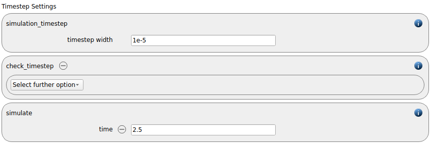
In this tab, we first define the time-step settings such as the desired simulation timestep of 1e-5 seconds and the total simulation time of 2.5 seconds. Per default also the check_timestep command command is enabled, which throws a warning when the time step exceeds 10 % of the Rayleigh or the Hertz time. These thresholds can be changed by setting an alternative value for hertz_fraction or rayleigh_fraction.

Here we can also set the enable_loadbalancing command command which allows Aspherix to handle core distribution, optimizing and speeding up simulations:

Output settings

In this tab we first define the timestep width for the file and the terminal outputs:

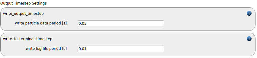
The output_settings command command the takes care that all particle information and the meshes are written to files accordingly. Furthermore it triggers the output of global quantities such as the kinetic energy of the particles or total normal and shear stresses onto meshes to the terminal. Please note that if the output of per-cell information on meshes such as wear, velocity of stress are desired, one has to add the keyword mesh_properties and select the required output.

Running the simulation

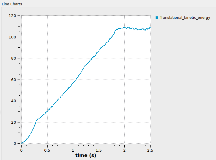
After completing the setup and saving it, the simulation can be launched. Change to the Simulation view. First hit the “Check settings” button, and if the check returns “Check settings successfully completed” the simulation can be run by hitting “Start”. The plots below show the kinetic energy and forces in the magnetic plate. The kinetic energy increases until the simulation reaches steady state after about 1.8 seconds:

Postprocessing with Paraview

After the simulation is completed, all data written with the output_settings command can be visualized automatically by going to the Visualization view and hitting the “Start Paraview” button.

The images below show the final state of the settled particles. The image has been rendered.