Battery Heating

In this tutorial we simulate the heating of a battery cathode following a compression which could for example be caused by an impact. In the first simulation a pack of particles is inserted, which undergoes step wise compression in the second simulation. The presence of an electric potential between the top and bottom plate leads to electric heating of the particle bed.

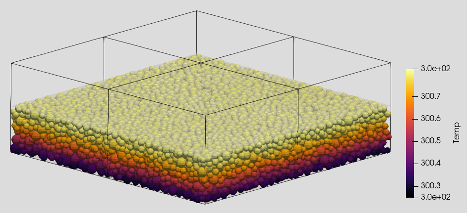
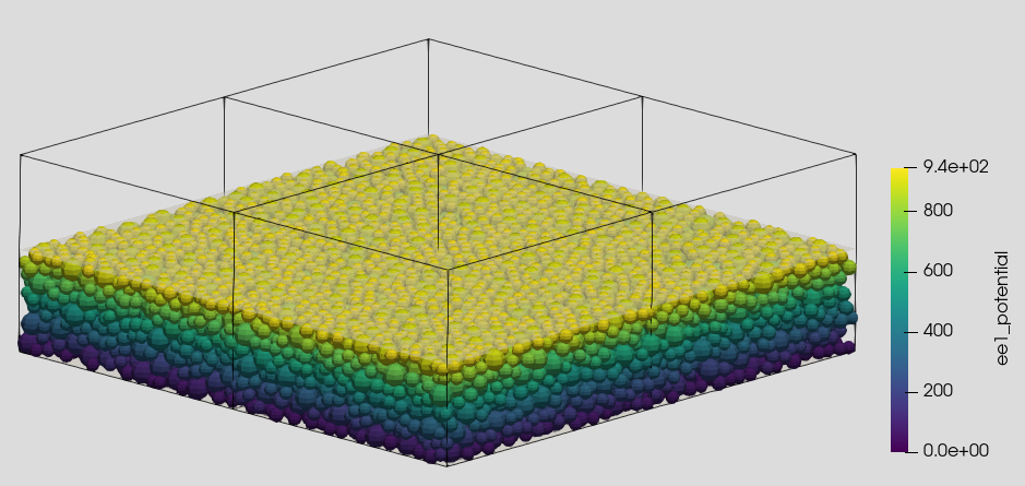
The images show the electric potential and the particle temperature at the end of the simulation:

Name of the case: Project_Battery_Heating

Case 1: Filling

In this case we are considering very fine powder and a small simulation domain. We therefore to to the Expert Settings tab and change from the default unit system (SI) to the micro units command:

Then, the used materials command as well as the simulation domain are defined in the General Settings tab. Please note that the dimensions of the simulation domain can only be defined in the first simulation. This means that the box that forms the simulation domain has to be chosen big enough from the beginning.

General settings

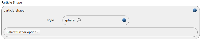
In this simulation we set particles of particle shape sphere:

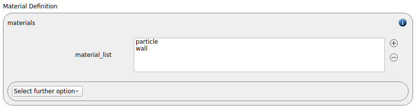
Two materials command are used:

The simulation domain is defined with x and y dimensions ranging from -150 to 150 micrometers, and z domain ranging from 0 to 103.75 micrometers.

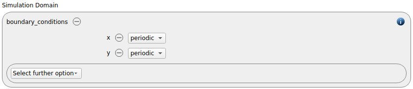
For mimicking an unconfined particle bed, we introduce periodic boundaries in x and y direction:

Meshes and regions

With respect to the z dimension the particle bed is confined by two meshes:

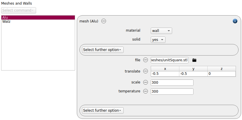
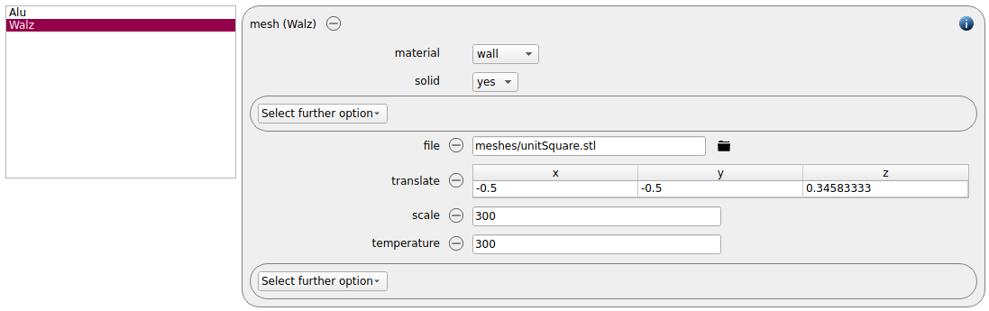
Since heat transfer will be actived in the next setup step, the meshes are both assigned a temperature.

Physics models

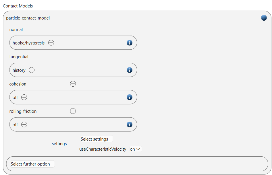
In the next step, the definition of the physics models takes place. For the particles we use the normal contact model hooke/hysteresis and the tangential model history.

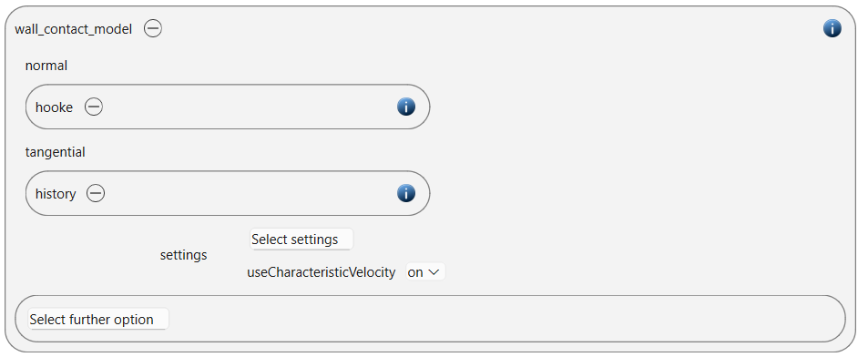
Since a wall mesh (the chute) was added in the previous section, a wall contact model is added automatically in this section. We use the hooke normal model and the tangential model history.

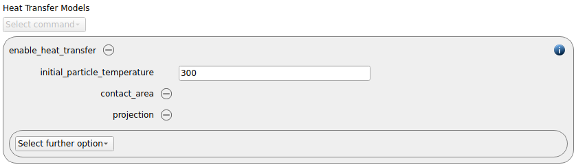
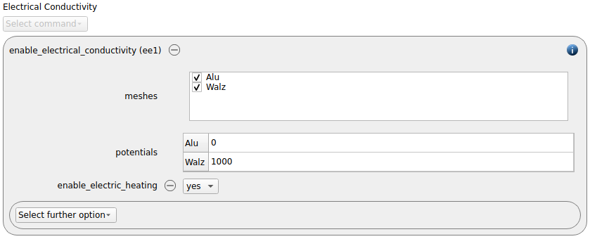
In this simulation, both heat transfer and electrical conductivity are active:

The enable_gravity command command is removed in this simulation.

Particles

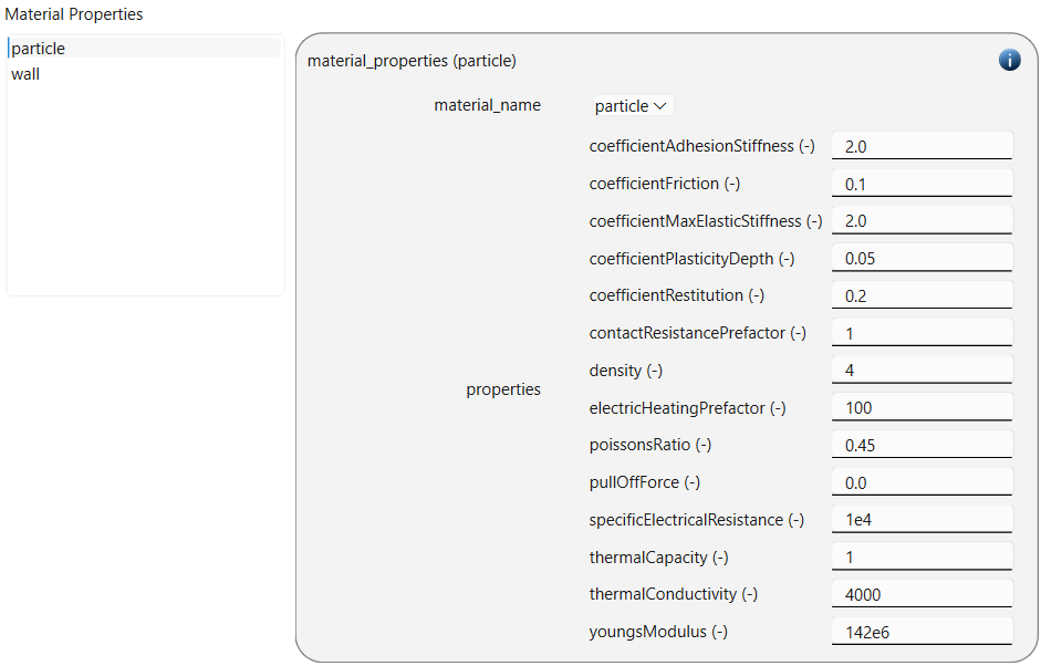
In the general settings tab we defined two material types (part and wall), whose material properties have to be specified here:

property	particle	wall
density	4.0	8.0
Young’s modulus	142e6	200e6
Poisson’s ratio	0.45	0.45
Coefficient of restitution	0.2	0.2
Coefficient of friction	0.1	0.1
Coefficient of maximal elastic stiffness	2.0	2.0
Coefficient of adhesion stiffness	2.0	2.0
Coefficient of plasticity depth	0.05	0.04
Contact resistance prefactor	1.0	1.0
Thermal capacity	1.0	1.0
Thermal conductivity	4000	4000
Electric heating prefactor	100	100
Specific electrical resistance	1e4	1e-6
pullOffForce	0	0

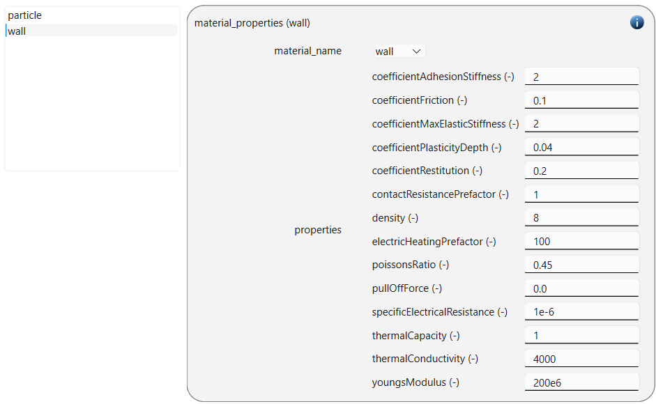
The material interaction properties are defined as following:

property	particle-wall interaction parameter
Coefficient of restitution	0.2
Coefficient of friction	0.1
Coefficient of maximal elastic stiffness	2.0
Coefficient of adhesion stiffness	2.0
Coefficient of plasticity depth	0.05
Contact resistance prefactor	1.0
Electric heating prefactor	100
pullOffForce	0

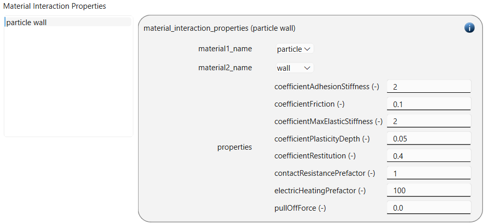
The hooke contact models also require the definition of a characteristiy velocity:

The granular material for this case consists of four different spherical particle templates of material particle with radii of 3.5, 4, 5 and 6 micrometers:

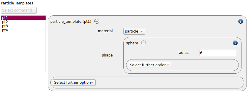
Based on this template a particle distribution is created:

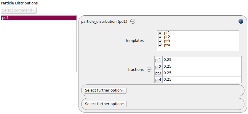
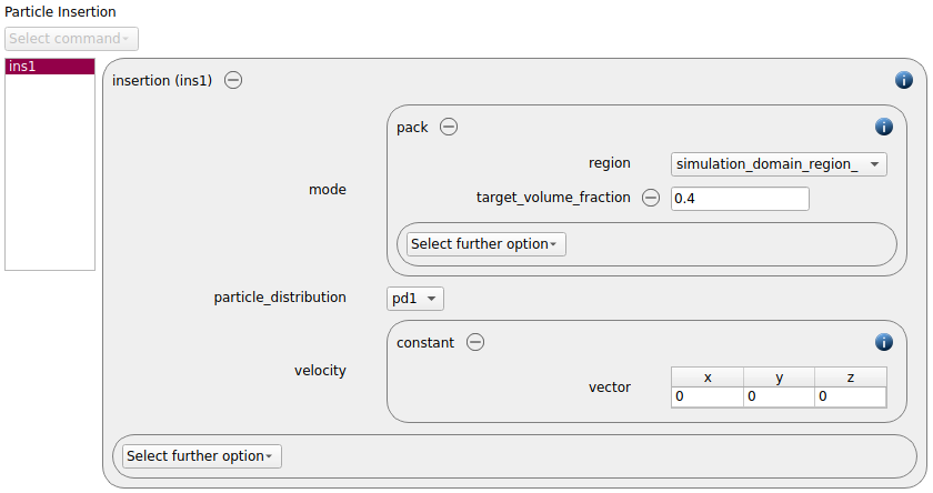
The final step in this tab is the definition of the insertion command. We of particles once at the beginning of the simulation, targeting for a volume fraction of 0.4. The initial velocity of the particles is defined as 0 in all directions:

Simulation control

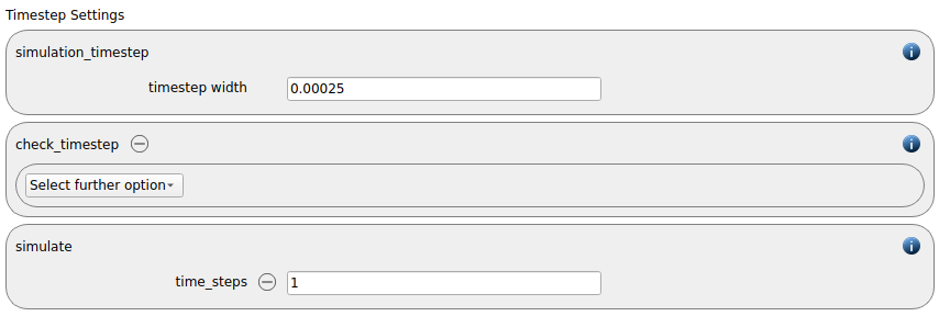
In this tab, one first choses the time step settings such as the desired simulation timestep of 0.00025 seconds. The filling simulation is only run for a single time step. Per default, the check_timestep command command is also enabled, which throws a warning when the time step exceeds 10 % of the Rayleigh or the Hertz time. These thresholds can be changed by setting an alternative value for hertz_fraction or rayleigh_fraction.

Loadbalancing is applied for an optimal usage of the computational resources:

Output settings

In this tab, we first define the timestep width for the file and the terminal output:

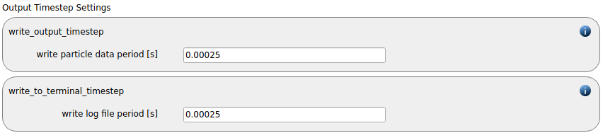
Since the simulation is only executed for a single time step, the output intervals are chosen equal to the simulation time step. This will be adapted in the following simulation to avoid excessive data output.

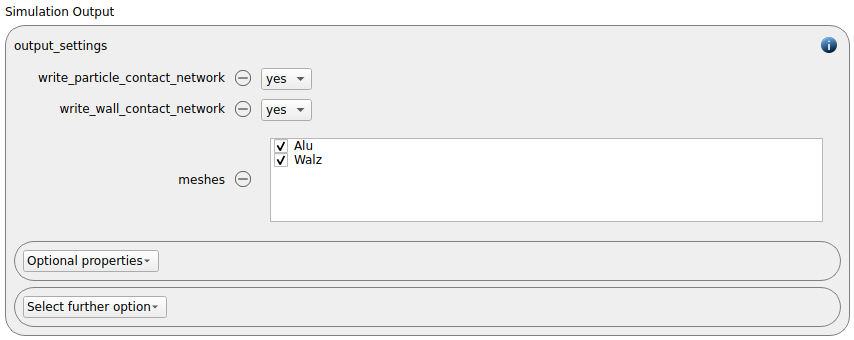
The output_settings command command takes care that all particle information and meshes are written to files. Furthermore, it triggers the output of global quantities such as the kinetic energy of the particles or total normal and shear stresses onto meshes to the terminal for those meshes that are selected:

Simulation

After completing the setup and saving it, the simulation can be launched. Therefore, change to the Simulation view. First hit the “Check settings” button, and if the check returns “Check settings successfully completed” the simulation can be run by hitting “Start”:

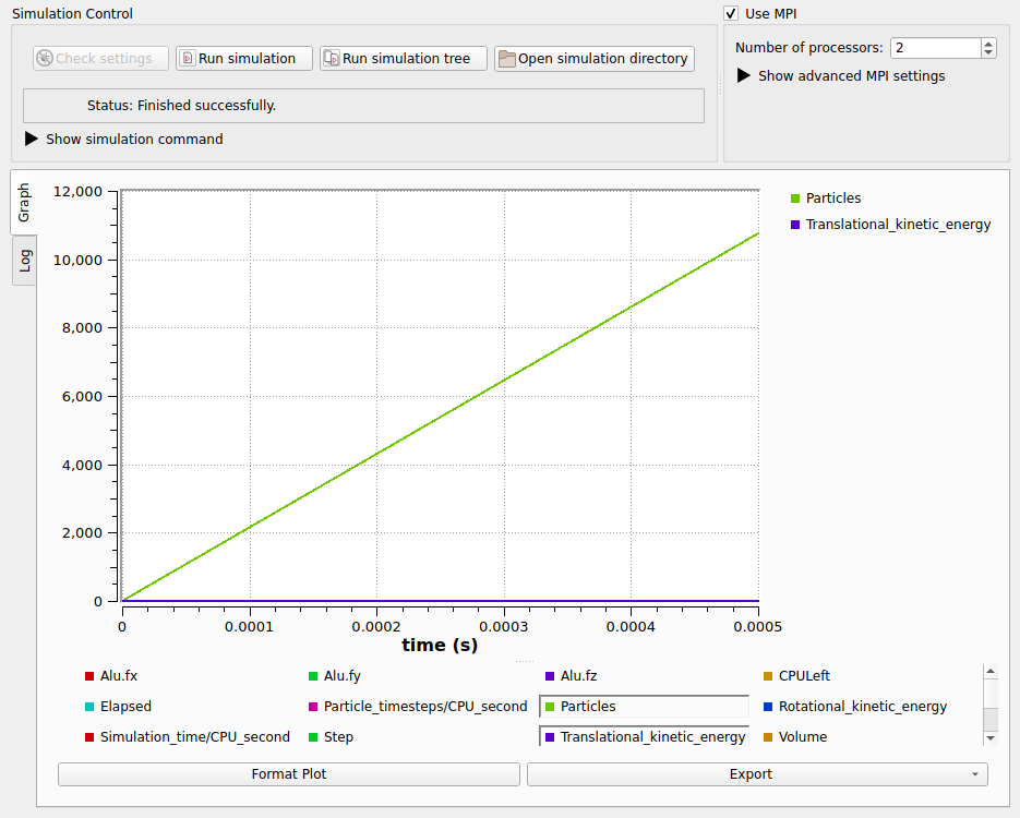
In this case the simulation is run on 2 cores, with a total of around 10000 particles this is a good choice also for the longer simulation later on.

Postprocessing

For postprocessing both Paraview and Ovito can be used.

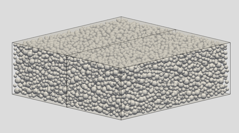
Particle bed in Paraview:

Case 2: Compression

In the second part of this case the particles are compressed in 2 phases, each of which is followed by a relaxation phase. The main focus lies on the average particle temperature of the particle bed during the process and its porosity.

Meshes and regions

After generating a dervied simulation, we start by adding a motion mesh module of type file.

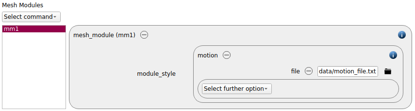
The goal is to move the top plate first for 8 and then of 2 microseconds with a velocity of 5 micrometers/microsecond in negative z direction. Each of the motion-phases should be followed by a resting phase of 5 microseconds. The corresponding motion file looks as following:

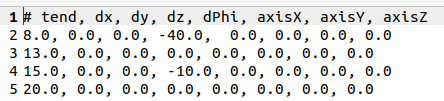
The first column consists in the end time of a respective motion, the following three columns contain the relative displacement in x, y and z direction since the last motion and the last four columns would be used to define an angle and an axis in case of a rotational motion.

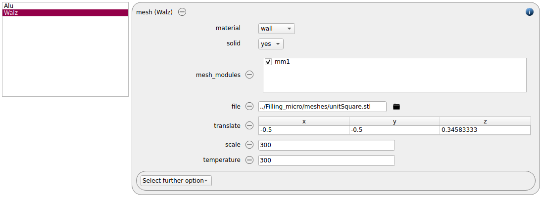
The mesh module now has to be added to the top mesh:

Particles

Next, please remove the insertion command from the particles section:

Simulation control

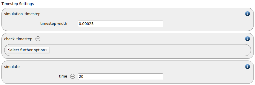
In the simulation control tab we change the simulation time from one timestep to a time of 20 microseconds.

Output settings

In the output settings tab we first increase the write_to_terminal_timestep to 0.1 microseconds and the write_output_timestep to 0.5 microseconds:

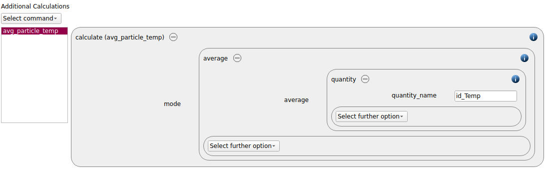
By introducing a calculate command command of type average we trigger calculation and output of the average particle temperature during the simulation:

Custom commands

For monitoring the porosity of the particle bed at run time, a few custom commands are required:

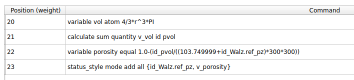
First, the volume of each particle in the packing is determined, then the volumes are summed up and finally the current volume between the two plates is divided by this result. For the calculation of the volume between the plates we use the z-position of reference point of the Walz mesh, which can be accessed by id_Walz.ref_pz, which is together with the porosity added to the global simulation output using the status_style command command.

Simulation

As soon as all modifications are completed the simulation can be launched:

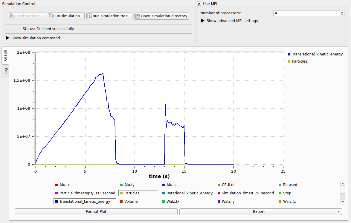
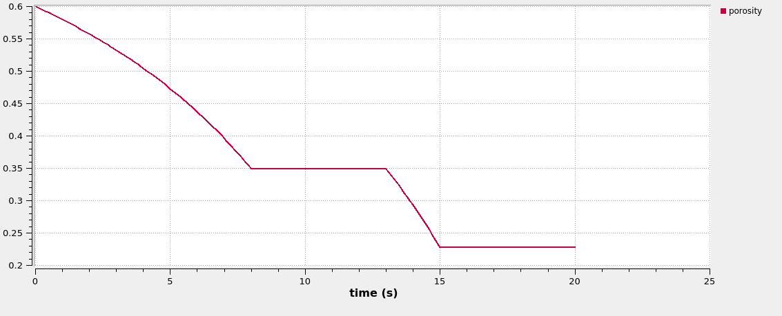
The kinetic energy of the particle bed already clearly shows the motion (particle compression) and resting phases. This is also reflected by the porosity of the bed:

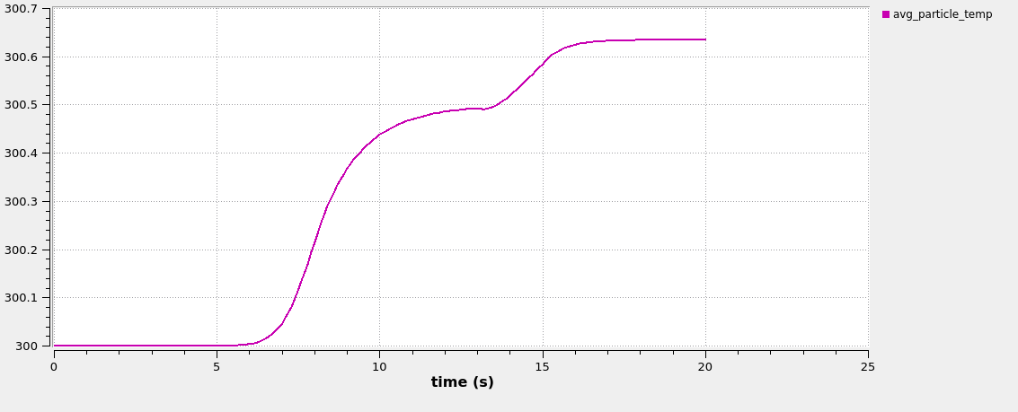
While lid position and porosity remain constant during the resting phases and increase of the particle bed can be observed due to electrical heating:

Postprocessing

The results can be postprocessed both in Paraview and Ovito. The images below show the results at the last time step, coloring is according to temperature and electric potential:

---