Melting of particles

In this simulation project we demonstrate the usage of a temperature-dependent melting model. In an initial simulation we fill a geometry, in the second step the particles are first colored by layers for better post processing and then we expose particles in a circular region to a temperature field (here a constant temperature field is chosen, but it could as well be a field stemming from a CFD calculation). The particles are heated up until they reach a defined melting temperature of 400K from which on they start to melt (shrink). As soon as a minimal particle size is reached, the particles are deleted entirely. For keeping the mass in the system (more or less) constant, new particles are inserted.

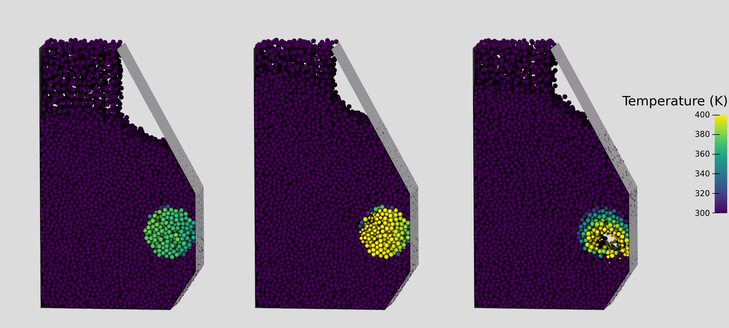
The image shows the state of the particle bed at three different times: first, the particles in the area where the temperature is applied heat up. They start to shrink once the melting temperature is reached, and when reaching a certain size they are removed entirely.

The testcase consists of three separate simulations.

Name of the case: Project_Melting_Particles

Simulation 1: Generate the particle packing

General settings

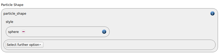
In this simulation we use particles of shape sphere:

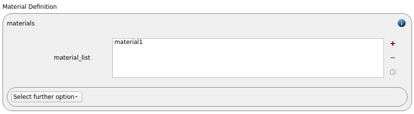
A material with name material1 is defined:

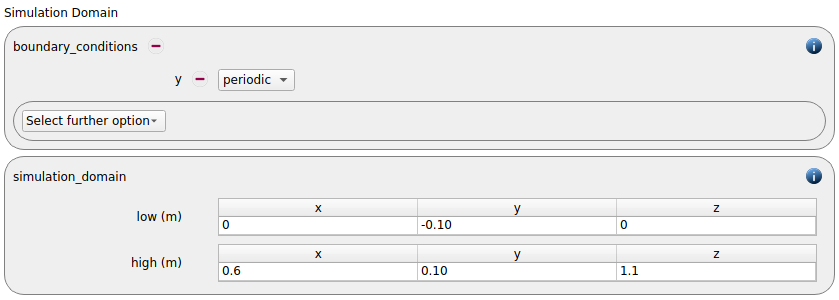
The simulation domain is defined with x dimensions ranging from 0 to 0.6 meters, y dimensions reaching from -0.1 to 0.1 meters and z dimensions ranging from 0 to 1.1 meters. For the xz-plane we use a periodic boundary.

Meshes and regions

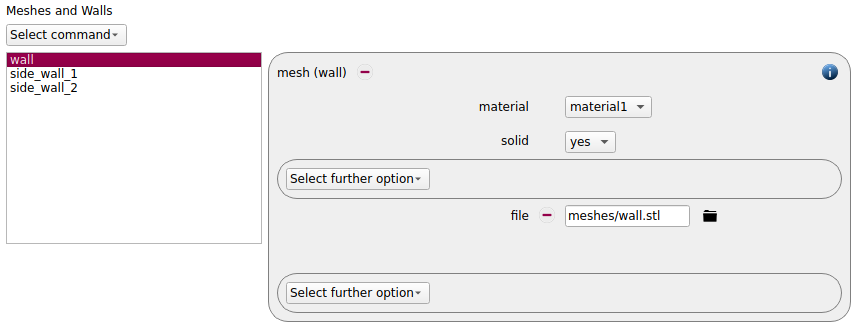
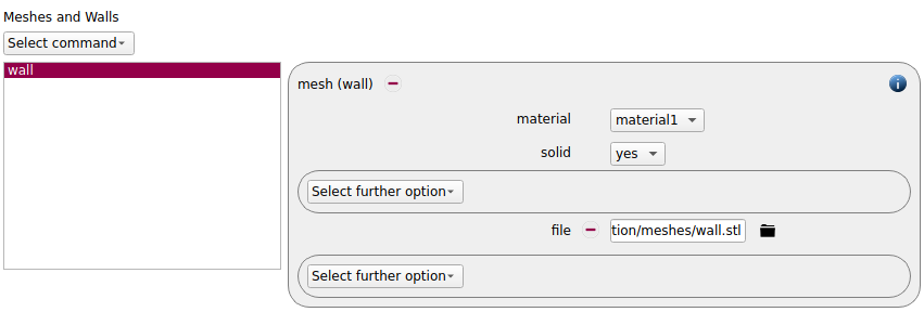
The geometry consists of a mesh command for the surrounding wall:

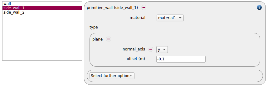
In this filling step two primitive walls are at the periodic boundaries:

name	normal_axis	offset
side_wall_1	y	-0.1
side_wall_2	y	0.1

This leads to an increased settling of the particle bed.

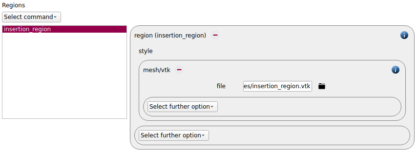
For the particle insertion we require an insertion region command:

Physics models

In the next step, the definition of the physics models takes place. For the particles we use the normal contact model hertz, the tangential model history and the rolling friction model epsd2.

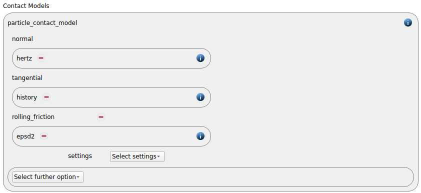
Since we added meshes in the previous section, also a wall contact model was added automatically in this section. We use the same contact models.:

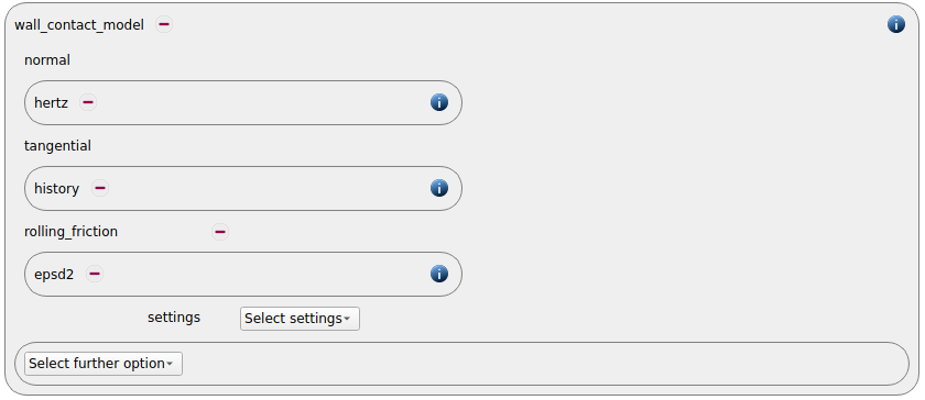
Finally also the gravity is defined:

Per default the gravity has a magnitude of 9.807 and acts into negative z-direction. These defaults can be changed by either setting the magnitude or the direction manually.

Particles

In the general settings tab we introduced one material. Here we define the required material properties.

	material1
Density	7000
Young’s modulus	5e6
Poisson ratio	0.3
Coefficient of restitution	0.4
Coefficient of friction	0.6
Coefficient of rolling friction	0.1

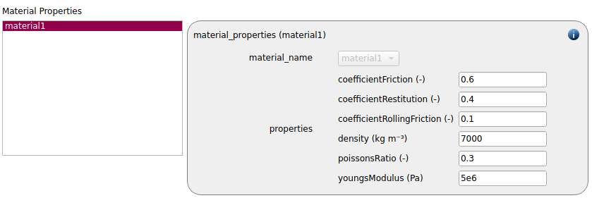
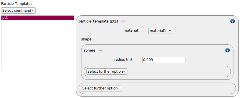
In the next step a particle template is generated. First we use a sphere-template, which only requires the definition of the radius:

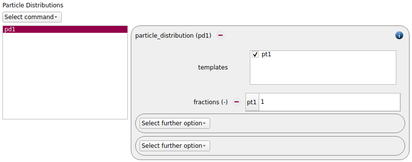
This template is used to define a particle distribution:

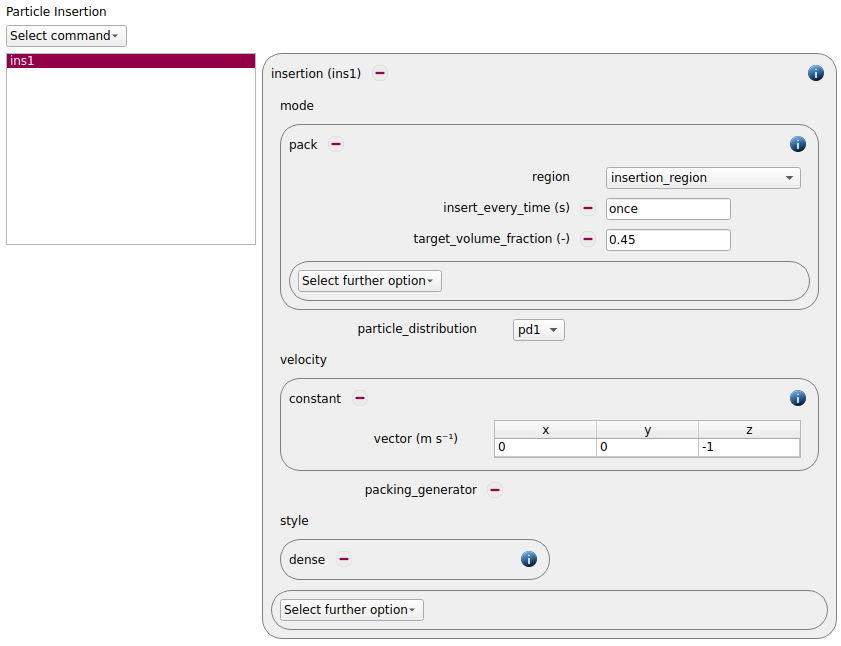
An insertion command command of type pack is used to insert particles into the previously defined insertion region:

Simulation control

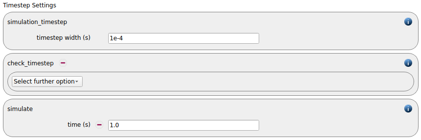
In this tab one first choses the time step settings such as the desired simulation timestep of 1e-4 seconds. With the simulate command we set the run time to one second:

For an optimal distribution of the loads on the processors we activate the

loadbalancing:

Output settings

In this tab we first define the timestep width for the file and the terminal output:

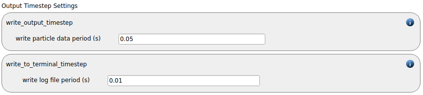
The output_settings command command takes care that all particle information and the meshes are written to files accordingly. Furthermore it triggers the output of global quantities such as the kinetic energy of the particles or total normal and shear stresses onto meshes in the terminal. Please note that if the output of per-cell information on meshes such as wear, velocity or stress are desired, the keyword mesh_properties has to be added and the required output has to be selected.

Running the simulation

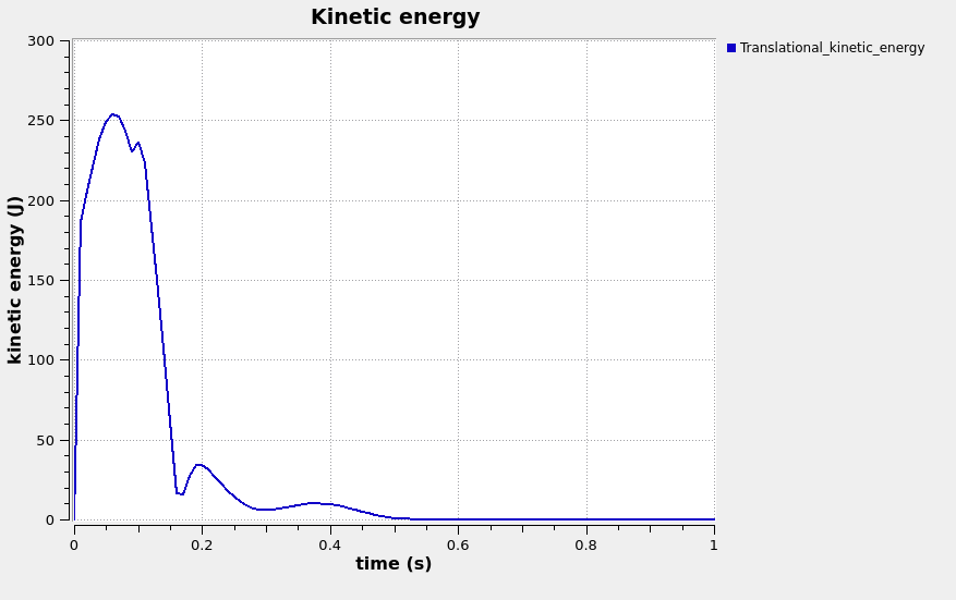
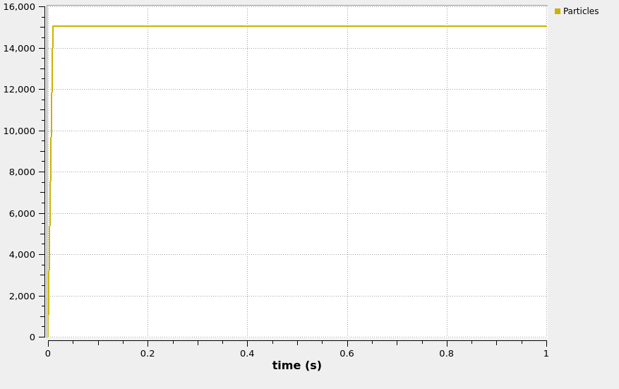
After saving the case we can change to the Simulation section. By hitting the Start button we can start running the simulation either serially or in parallel, using mpi. Number of particles, kinetic energy, number of particles as well as the forces on the geometry components can be visualized.

Result

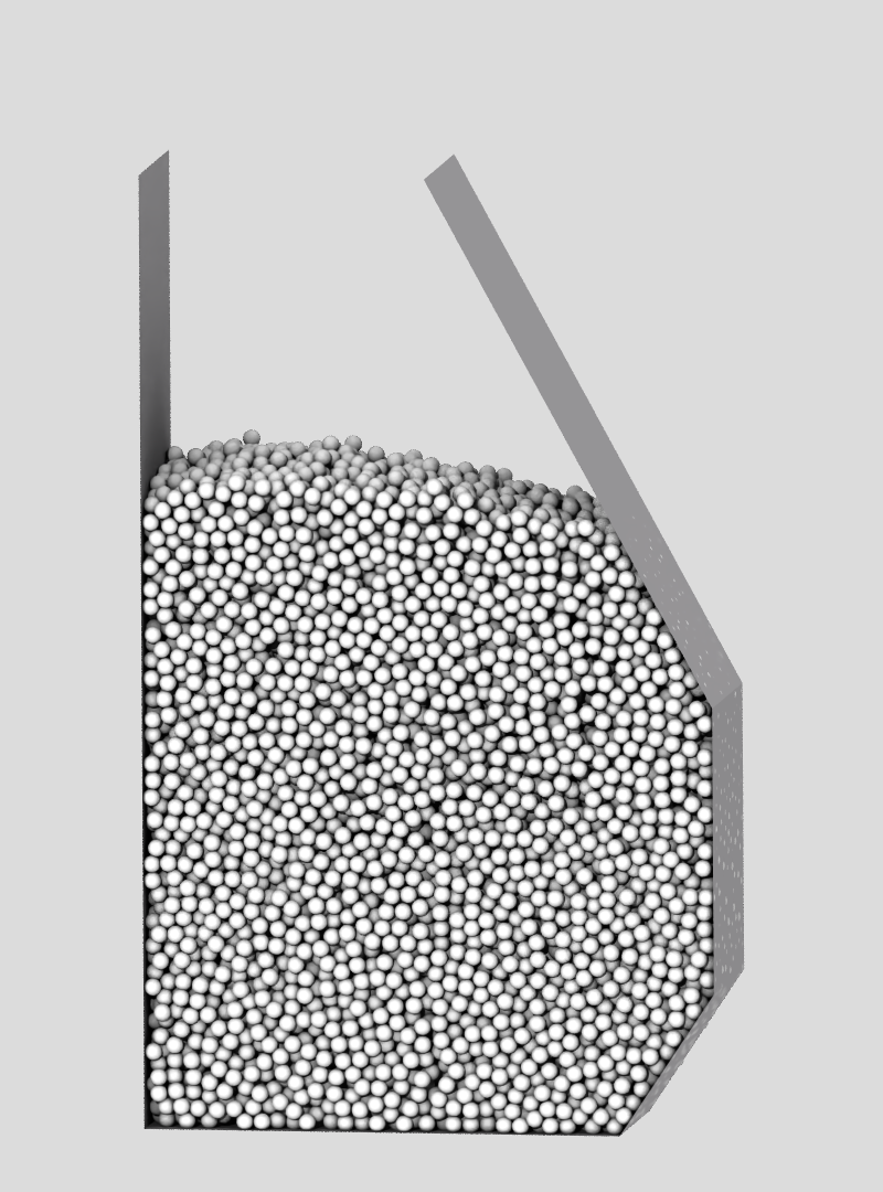
The result of the calculation can then be visualized with Paraview. The image shows the particles colored according to their radius.

Simulation 2: Melting

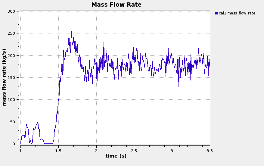
In this simulation one-way coupling against a temperature field from a fluid is used to heat up particles in a defined region. In the course of melting, the particles become smaller and are finally deleted. This induces a massflow towards the melting region which is measured with a calculate command.

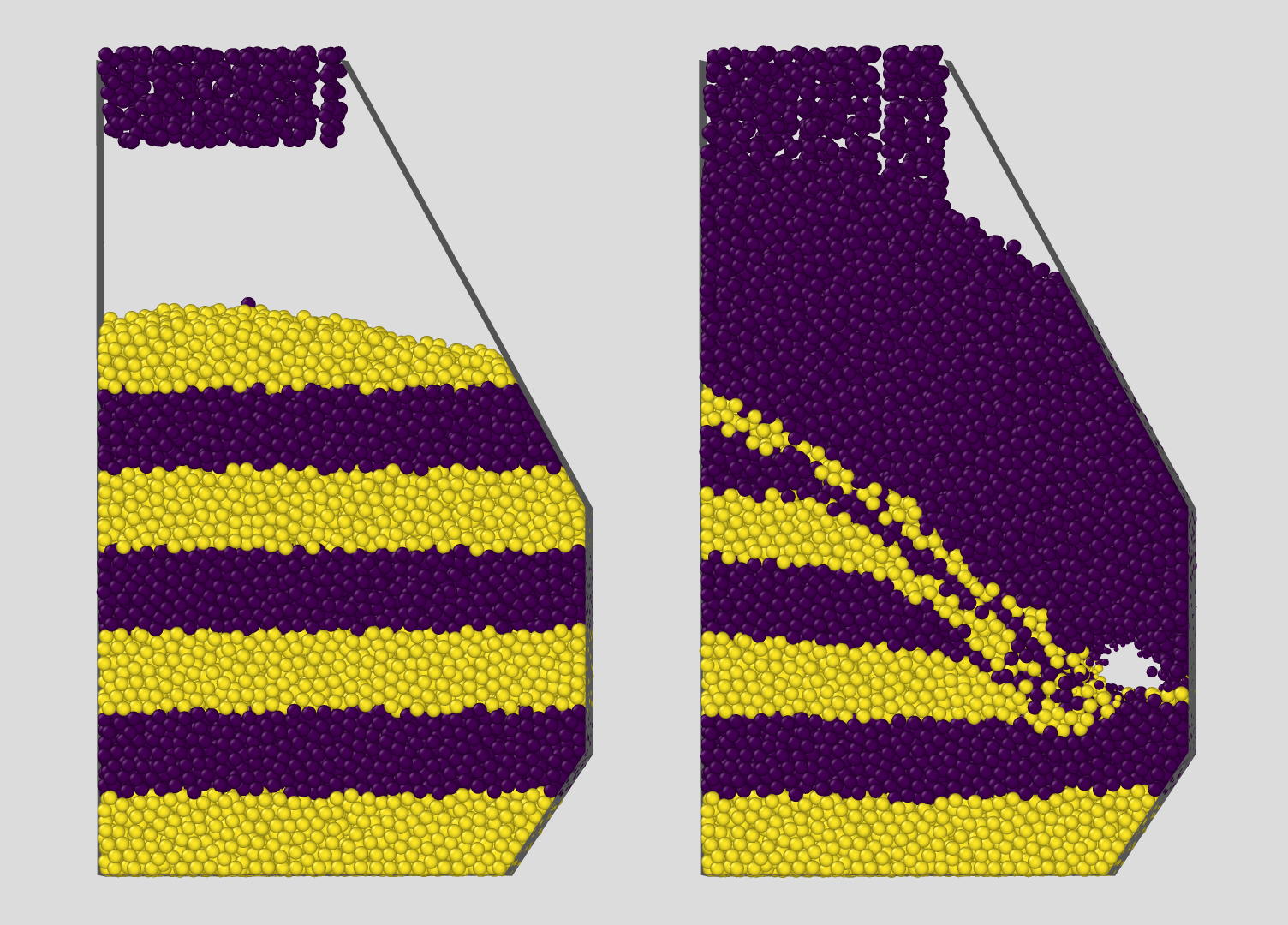
For a better visualization of the bed motion we mark particles layer-wise.

apply different colors to particles in different regions for an easier postprocessing later on. Furthermore, the insertion command is removed.

Meshes and regions

The two primitive walls at the periodic boundaries are removed:

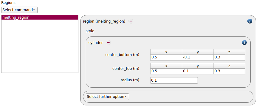
The insertion region from before is replaced by a cylindric melting_region:

Physics models

Both the enable_particle_melting command and the enable_heat_transfer command command are added:

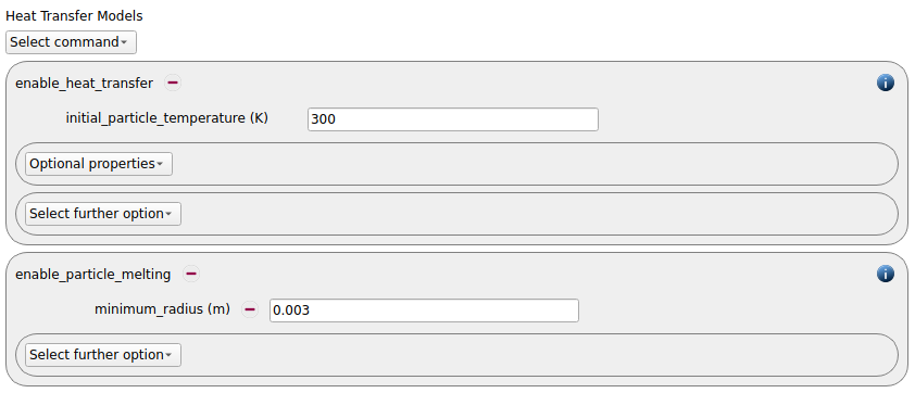
The initial particle temperature is set to 300K, the minimal particle radius is set to 0.003 m. Once the melting would cause the particles to become smaller than that they will be removed from the simulation.

Particles

With the addition of the melting model four new material properties are required, namely the thermal conductivity, the thermal capacity, the latent heat and the melting temperature.

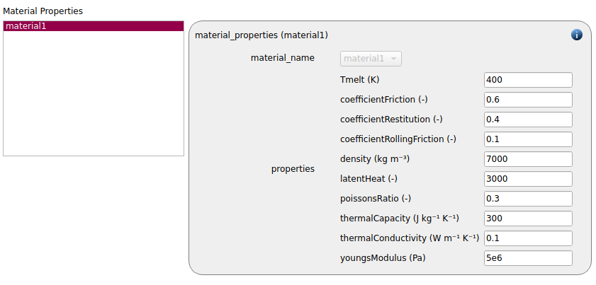
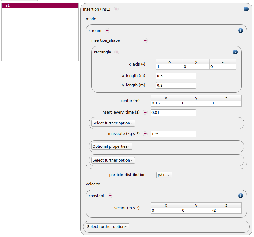
Furthermore, also a the insertion is changed to type stream:

For marking particles in layers, we first define four groups that define four layers through a condition:

name	condition
dg1	z<0.1
dg2	z>0.2&&z<0.3
dg3	z>0.4&&z<0.5
dg4	z>0.6&&z<0.7

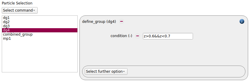
These four groups are united to one:

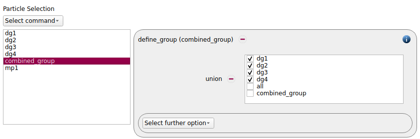
This group is then used in the mark_particles command command:

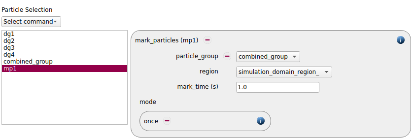
Coupled simulation

The enable_one_way_coupling command command is used to introduce a one-way coupling. We are using a velocity field that is zero everywhere:

x y z U_x U_y U_z
0.1 0 0.1 0 0 0
0.5 0 0.9 0 0 0

The temperature field has a constant temperature of 450K:

x y z T
0.1 0.05 0.1 450
0.5 0.05 0.9 450

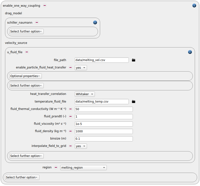
Please make sure that the option “interpolate_field_to_grid yes” is used at all times. Without this option only velocity / temperature fields can be used that contain data at exactly every bin, and such fields are very hard to obtain. Please make sure that your velocity / temperature fields are fine enough (when non-constant the distance between the points should be approx. the bin size) because a simple interpolation algorithm is applied that can lead to unexpected results when too coarse fields are used.

Simulation control

Since the particle size changes due to the melting, the time step width is reduced to 5e-5 seconds, and the run time is set to 2.5 seconds:

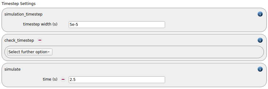
Output settings

For obtaining the massflow that is induced by the particle melting, a calculate massflow command is used:

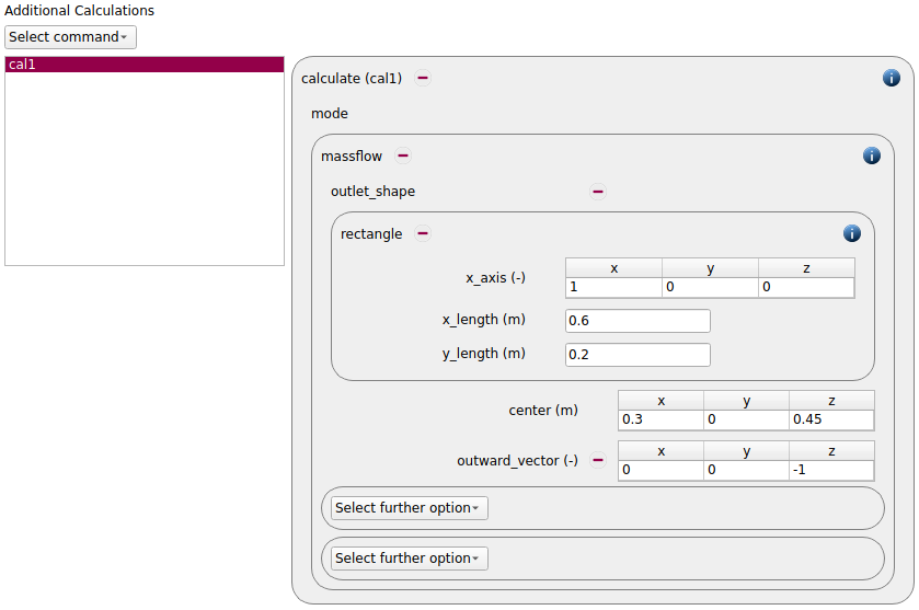
The output_settings command automatically makes sure that the results can be visualized in the graph during the simulation.

Running the simulation & postprocessing

Again the simulation can be launched, e.g., on 4 processors.

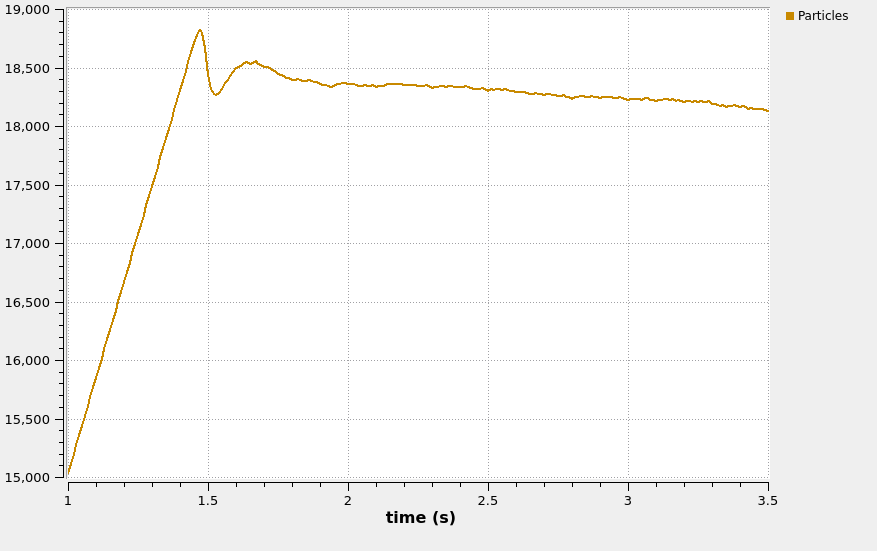
The graphs below show the the number of particles as well as the massflow rate through the plane:

The results can also be visualized in paraview. This image shows the particle bed according to the different layers at different time steps:

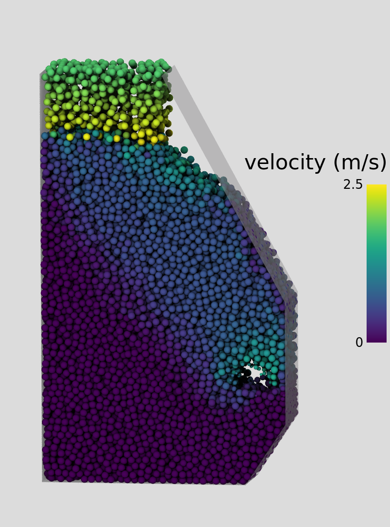
In this image the particles are colored according to their velocity (at the last time step):

The image shows the state of the particle bed at three different times: first, the particles in the area where the temperature is applied heat up. They start to shrink once the melting temperature is reached, and when reaching a certain size they are removed entirely.