Compressing Particles

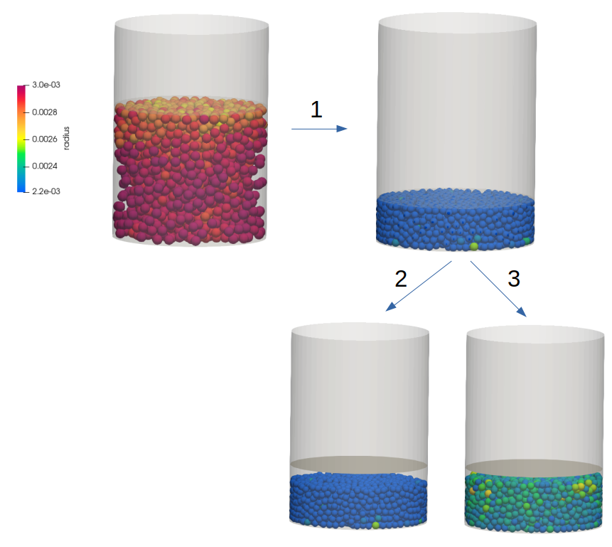
In this simulation project we first insert particles in a cylindric region and use a force- controlled servo wall to compress the packing (1). The powder compression model fix powder/update that is applied allows for a plastic deformation of the particles and thus a strong increase of the bluk density of the material. The second step we decompress the bed by exchanging the force controlled wall by a velocity controlled wall that moves up slowly. In one case we use the same parameters as the for compression case (2), in the other case we activate the elastic dilation (3).

This image shows the intial state of the simulation during compression, the compressed particle bed and the two final decompressed particle beds for the different parameters:

For obtaining particular compression curves a hardening model can be used within the frame of this powder compression model.

Name of the case: Project_Compress_Particles

Case 1: Particle Compression

General settings

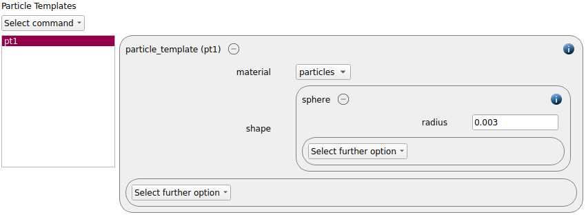
In this simulation we use particles of particle_shape command sphere:

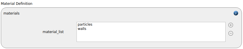
Two materials command named particles and walls are generated:

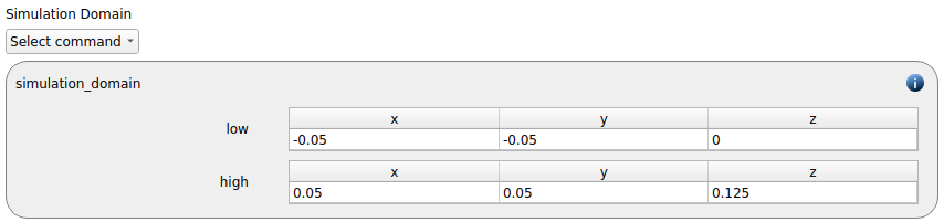
The simulation domain is defined with x and y dimensions ranging from -0.05 m to 0.05 m, and z dimensions ranging from 0 to 0.125 meters:

Meshes and regions

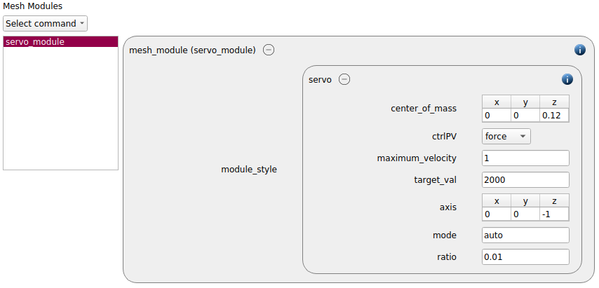
We use a force controlled mesh for compressing the particles, so we start with the definition of a a mesh_module of type servo. The center of mass if set to (0, 0, 0.12) since the top wall will be inserted at a height of 0.12 m. The crtlPV mode “force” is selected and the target value is 20000. As axis we use the negative z axis. The maximum velocity is set to 1 and the ratio to 0.01:

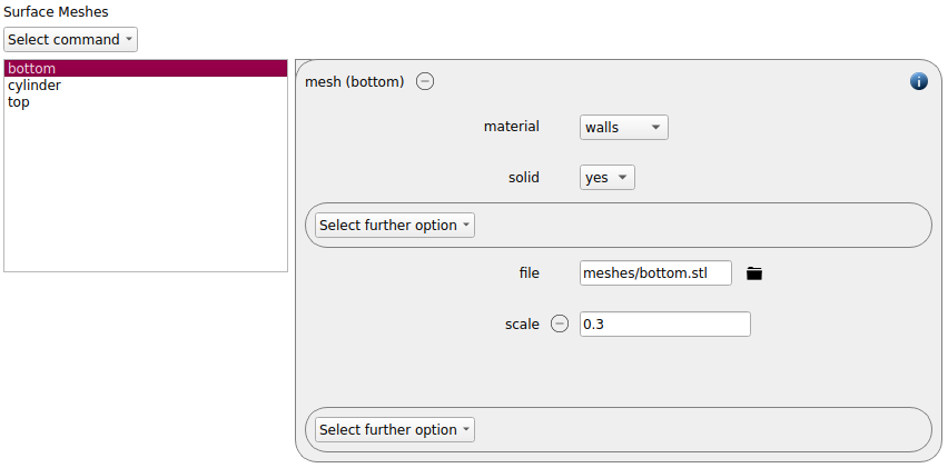
The we proceed with loading the meshes. First the bottom plate is added. As all other meshes in this project it is of type solid, i.e., it is used as wall. We apply a scaling factor of 0.3 to it.

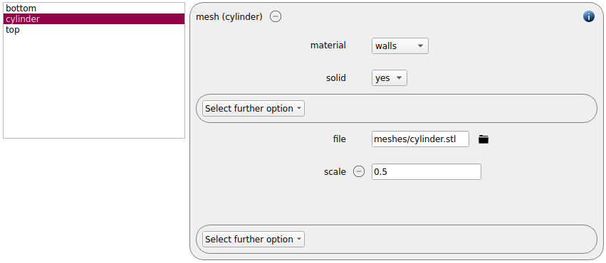
Then the cylindric wall is loaded, with a scaling factor of 0.5:

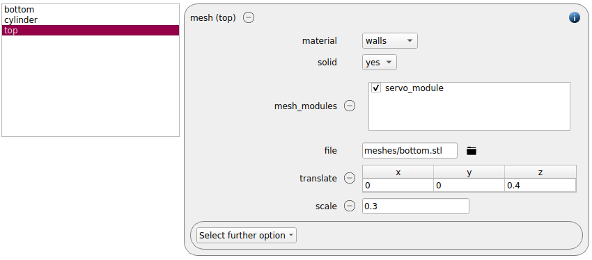
Finally, we insert the top wall. We use the same mesh file as for the bottom, but translate it by 0.4 m in z direction. Since the translation is applied before the scaling the initial height of the top wall is 0.12 m. We also apply the servo mesh module to this geometry component:

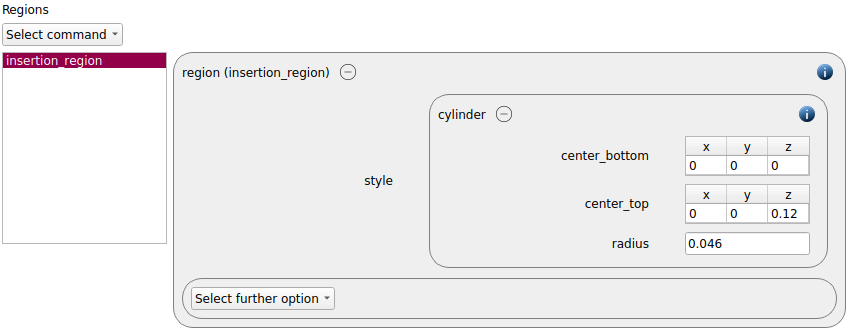
We want to insert particles inside the cylinder only, so we define a region of style cylinder. The bottom center is (0, 0, 0), the top center is (0, 0, 0.12) and the radius is 0.046 to make sure that no particles get stuck in the meshed walls.

Physics models

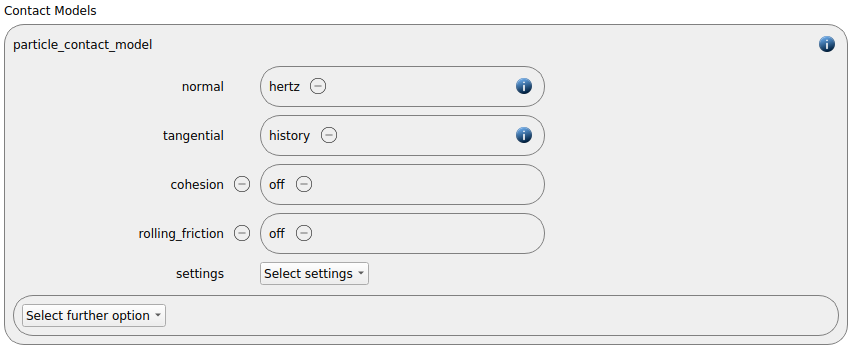
In the next step, the definition of the physics models takes place. For the particles we use the normal contact model hertz and the tangential model history.

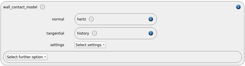
Since we added meshes in the previous section, also a wall contact model was added automatically in this section. We use the same contact models as for the particles:

In the section “Advanced Contact Models” we select the fix powder/update command to activate the powder compression model:

Finally also the gravity is defined:

Per default the gravity has a magnitude of 9.807 and acts into negative z-direction. These defaults can be changed by either setting the magnitude or the direction manually.

Particles

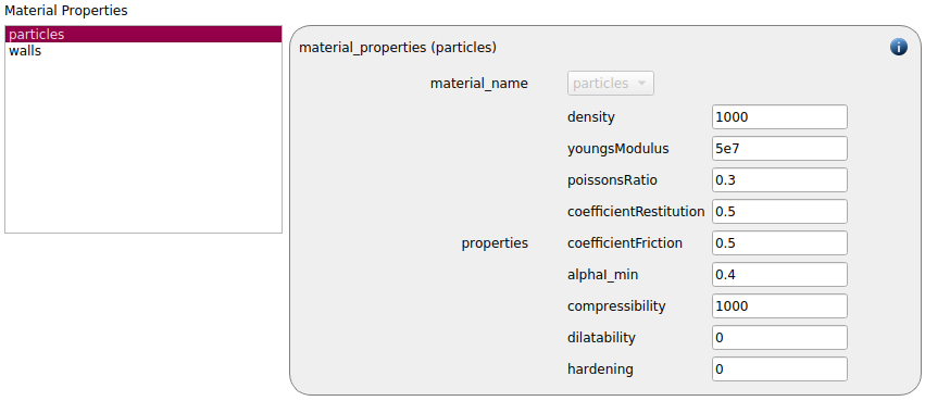
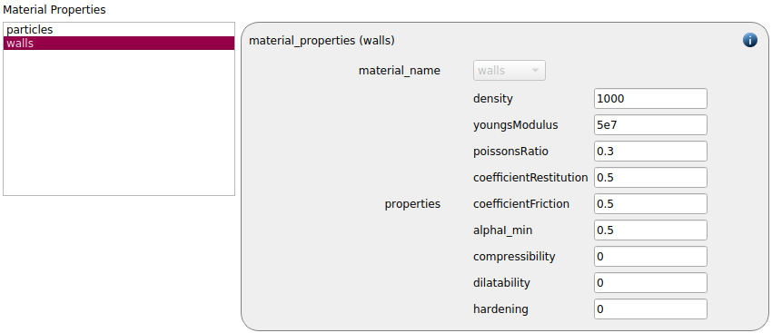
In the general settings tab we introduced two materials. Here we define the required material properties.

	particles	walls
Density	1000	1000
Young’s modulus	5e7	5e7
Poisson ratio	0.3	0.3
Coefficient of restitution	0.5	0.5
Coefficient of friction	0.5	0.5
asphaI_min	0.4	0.4
Compressibility	1000	0
Dilatability	0	0
Hardening	0	0

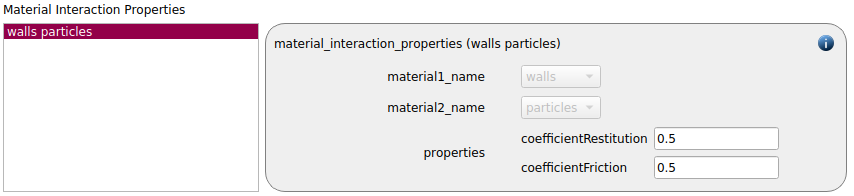
Next, the :doc:` material interaction properties <solver:material_interaction_properties>` are defined:

In the next step a particle template is generated:

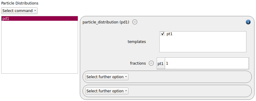
This template is used for a particle distribution:

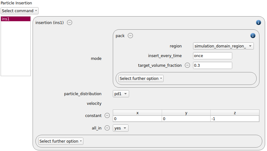
An insertion command command of type pack is used for the particle insertion. We use the previously defined insertion region and chose a target volume fraction of 0.3. The initial velocity of the particles is set to 1 in negative z-direction. The option “all_in yes” ensures that all particles are entirely inside the insertion region (“all_in no” means that all particle centers are inside the insertion domain, which could lead to particles getting stuck in the meshes walls).

Simulation control

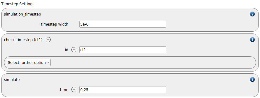
In this tab one first choses the time step settings such as the desired simulation timestep of 5e-6 seconds and the total simulation time of 0.25 second. Per default also the check_timestep command command is enabled, which throws a warning when the time step exceeds 10 % of the Rayleigh or the Hertz timestep. These thresholds can be changed by setting an alternative value for hertz_fraction or rayleigh_fraction. Please note that we have added an ID for the check_timestep command. This allows us to access the output values of the command (hertz and rayleigh timestep fraction) in the custom command section later on. If no custom output commands are used, this step is not required.

The enable_loadbalancing command command is used to ensure the highest efficiency for parallel runs.

Output settings

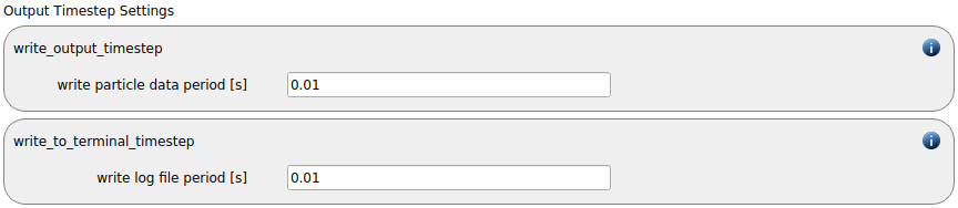
In this tab we first define the timestep width for the file and the terminal output:

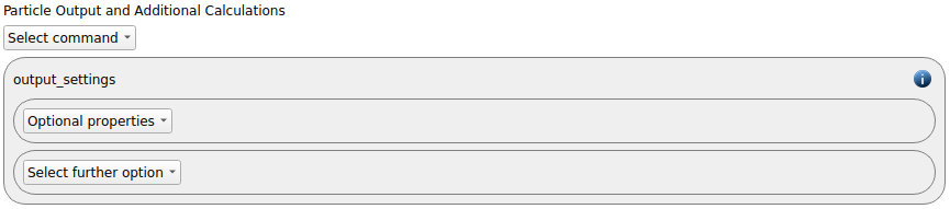
The output_settings command command takes care that all particle information and the meshes are written to files accordingly. Furthermore it triggers the output of global quantities such as the kinetic energy of the particles or total normal and shear stresses onto meshes in the terminal. Please note that if the output of per-cell information on meshes such as wear, velocity or stress are desired, the keyword mesh_properties has to be added and the required output has to be selected.

Custom settings

In our case, we are not only interested in automatically evaluated quantities such as the kinetic energy, but we would also like to know the current z-position of the top plate, the bulk density underneath the please and the average particle radius. These quantities can be calculated using custom commands, and with the aid of the status_style command command they can also be visulized in the graphs during the simulation.

1: Calculation of the average particle radius

First, we define a variable command of type atom such that we can access the radius of all particles. The user-defined name of the variable is rad, the fact that the r saves the radii of all particles can be found in the documentation of the variable command.

[weight 22] variable rad atom r

Then we use a reduce command to calculate the average of the variable rad. Variables are accessed via v_[variable name]:

[weight 23] reduce ave v_rad id averageRadius

The average particle radius is now calculated and it can be accessed through id_averageRadius in the status_style command or in the write_to_file command command.

2: Calculation of the bulk density

We would like to calculate the bulk density of the material underneath the top plate. Therefore we need the mass of all particles as well as the z-position of the plate. The radius of the cylinder is 0.045 m. This time, we use a variable of equal style for the calculation:

[weight 22] variable bulkDens equal mass(all)/(0.045*0.045*PI*id_top.zcm)

The group variable mass(all) and the expression PI are defined in the documentation of the variable command. The center of mass of meshes with the servo mesh module can be accessed (doc access) through xcm, ycm and zcm (see documentation of the mesh module servo).

3: Plotting the new quantities

We use the status_stlye command to overwrite the automatically generated status output that comes from output settings. We are displaying the following quantities:

expression	explanation
time	simulation time (s if SI units used)
step	time steps (time/dt)
atoms	number of particles
ke	kinetic energy within the system
id_rke	rolling kinetic energy
cu	Cundall number
id_ct1.hertz	Hertz timestep fraction
id_ct1.rayleigh	Rayleigh timestep fraction
id_top.zcm	z-center of mass of top wall
v_bulkDens	bulk density underneath top wall
id_averageRadius	average particle radius

[weight 24] status_style all {time,step,atoms,ke,c_rke,cu,id_ct1.hertz,id_ct1.rayleigh,id_top.zcm,v_bulkDens,id_averageRadius}

Note: The weights determine the order in which the commands are added to the autogenerated input script for the simulation. In this case is is important, that the variable for the radius is defined before the calculation of the average value and that the average radius and the bulk density exist when using the status style command. Since the latter is used to overwrite the automatic status generated by the output_settings command (which has weight 23 internally) its weight must be larger than that. All commands that should be executed during the simulation run must have weights smaller than 26.

Finally, the command section of the custom settings looks as following:

Running the simulation

Due to the low number of particles is is sufficient to run the simulation on two cores (Use MPI is active, Number of processors: 2).

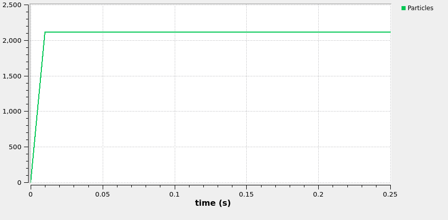
The graph shows that particles are inserted at the beginning and that the number of particles remains constant during the simulation:

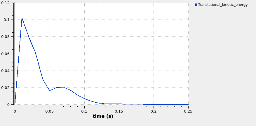
The kinetic energy of the system drops rapidly:

The following graphs show the bulk density, the z-position of the top plate and the average particle radius:

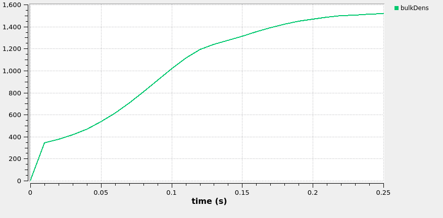
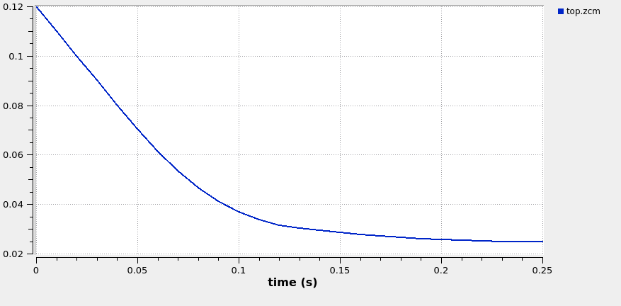
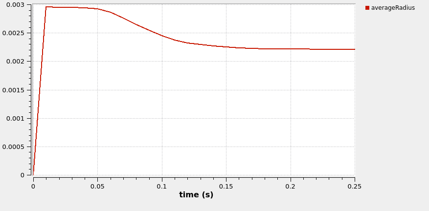
All these quantities have reached a plateau, indicating that the simulation has reached a steady state.

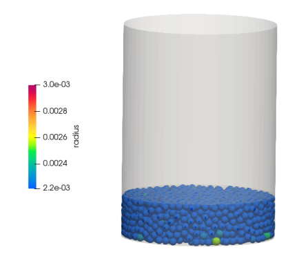
The compressed bed looks as following (coloring according to particle radius):

Case 2: “Decompression”

In this second simulation we are slowly releaseing the weight from the particle bed by moving the top plate up slowly. As a result the particle bed expands, the overlaps between the particles reduce due to the missing compression force. In this case, no elastic dilatation is permitted, so the radii of the particles remain constant over the simulation.

We start with deriving a simulation from the previous project by clicking on the “derive simulation”-button:

A new simulation project is created, based on the settings and results of the filling & compressing simulation.

The main tasks now consist in replacing the mesh module servo by a mesh module of type motion and by removing the insertion command, and as a consequence also the particle distribution, the particle template and the insertion region.

Since meshes with mesh module motion do not store the center of mass, the custom commands must be modified as well.

Meshes and regions

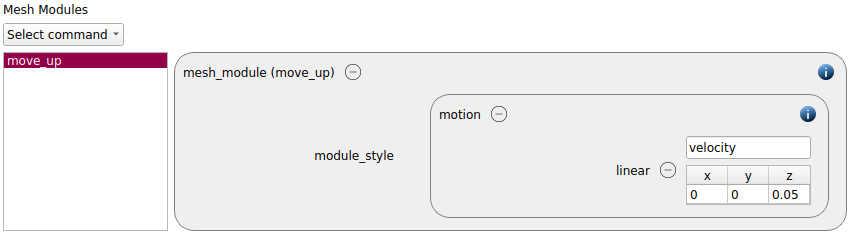
First of all we delete the mesh_module servo and create a new mesh_module of type motion:

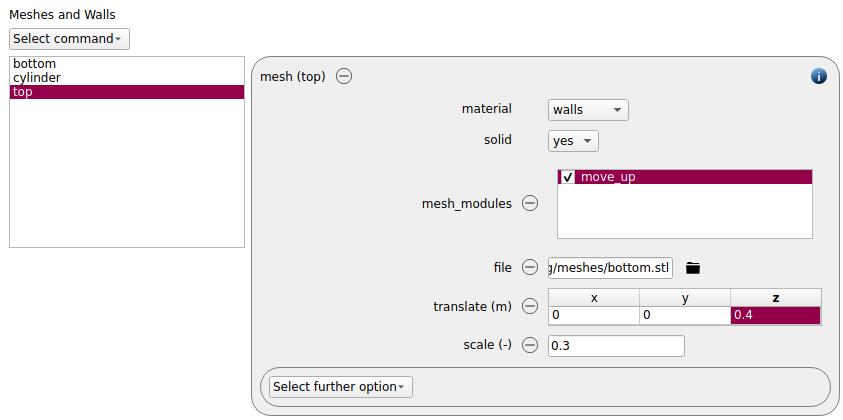
Please make sure that this mesh module is added to the top mesh accordingly:

The insertion region can be deleted.

Particles

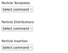
The insertion command, the particle distribution and the particle template can be deleted (in exactly this order):

Custom settings

Since the top mesh has no servo module any more, its center of mass is no longer stored. Furthermore, the mesh is moved upwards at a linear velocity, and its position is no longer representative for the bed volume. We will therefore remove the calculation of the bulk density and also remove the z-position from the status style.

The new status style command reads as following:

[weight 24] status_style status_style all {time,step,atoms,ke,id_rke,cu,id_ct1.hertz,id_ct1.rayleigh,id_averageRadius}

Running the simulation

Again, the simulation can be run with two processors.

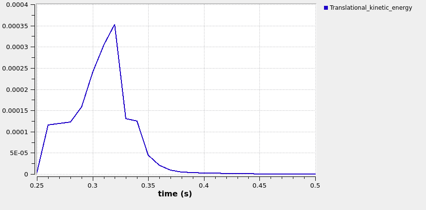
The plot with the kinetic energy shows that the simulation runs long enough for the bet to settle again after the decompression:

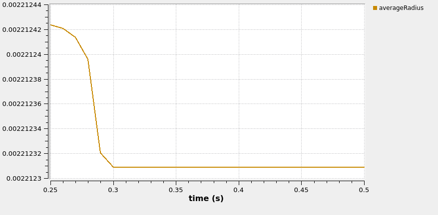
The average radius remains constant througout the entire simulation run (please note that the values on the y-axis cover a very small span):

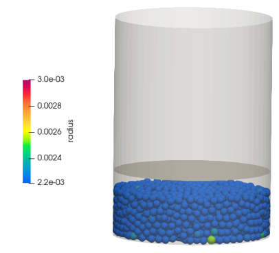
The expanded bed looks as following:

Case 3: “Decompression” with elastic dilation

This third simulation is a copy of the second one, with the main difference that elastic dilatation is switched on now. So apart from the expansion of the bed due to the reduction of the particle-overlaps the bed expands as well because of an elastic expansion of the particles once the force from the top plate is removed.

We use the “Clone simulation” button for generating a new simulation which is also based on the filling and compressing simulation:

Physics models

To allow for the elastic dilation the “elastic_dilatation” switch is set to yes:

Particles

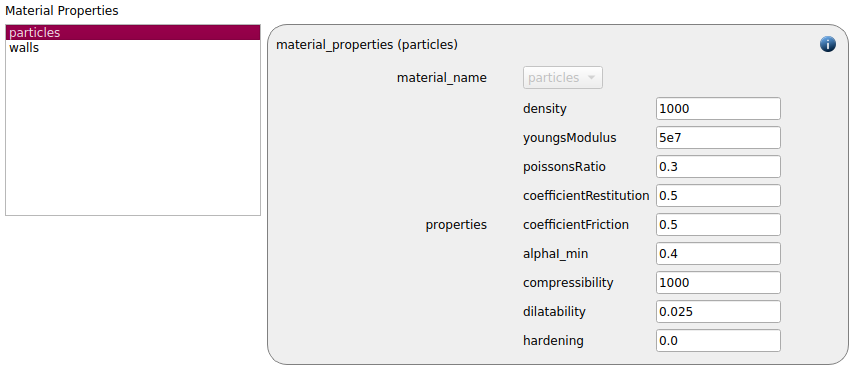
We change the dilatability parameter for the particles-material from 0 to 0.025:

All other modifications with repect to the base simulation (motion instead of servo, removal of insertion, particle distribution, particle template, insertion region, …) were done in simulation 2 already and do not have to be redone. We can move forwards to running the simulation right away.

Running the simulation

After running the simulation (e.g., on two processors) we get the following graphs for the kinetic energy and the average particle radius:

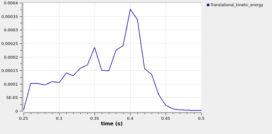
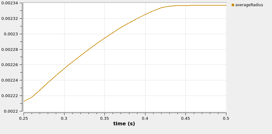
It becomes apparent that the particles’ radius increases when the force exerted by the top plate is removed. This also shows when postprocessing the results in Paraview: