 Home
HomeTablet press
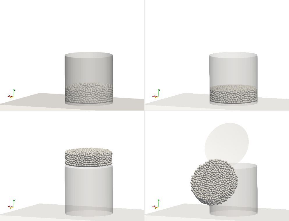
In this tutorial we model a tablet pressing process in four steps: first, granular material is inserted in a cylinder, then the powder is compacted to a tablet. In the last two steps the pressure onto the tablet is release and the tablet is ejected in two steps. A specific powder model is used which allows for the compaction of the material and which provides the required cohesion for creating a stable tablet.
Name of the case: Project_Tablet_Press
Case 1: Filling
As a first step, the particle shape, the used materials command and the simulation domain are defined in the General Settings tab.
General settings
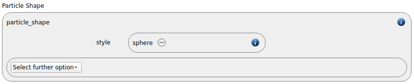
In this simulation we set particles of particle shape sphere:
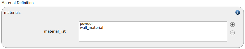
Two materials command “powder” and “wall_material” are used:
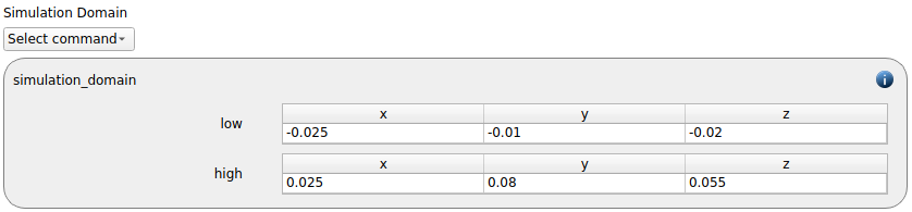
The simulation domain ranging from -0.025 to 0.025 in x, from -0.01 to 0.08 in y and from -0.02 to 0.055 in z direction is created:
Meshes and regions
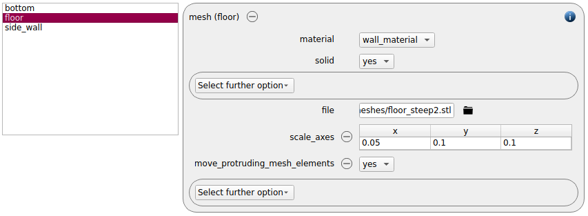
Three meshes are inserted, one for the side walls of the cylinder, one for the bottom shape of the tablet and a floor. Please note that the floor exceeds the simulation domain. By setting the keyword “move_protruding_mesh_elements” to “yes” we enforce Aspherix to ignore all mesh elements that are outside the calculation domain. All meshes are of “wall_material”:
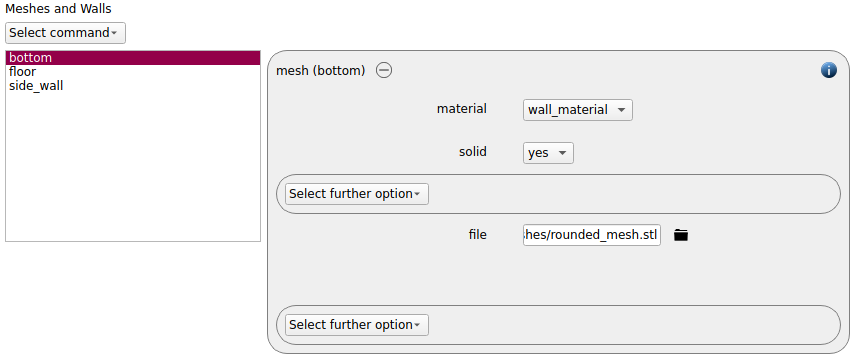
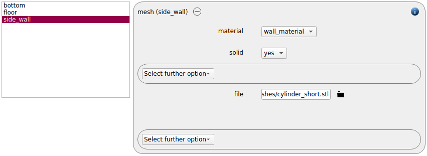
The floor mesh is scaled by a factor of 0.5 in x direction and by 0.1 in y and z direction:
Physics models
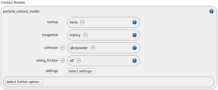
The contact models are now defined. For the particles we use the normal contact model hertz and the tangential model history and the cohesion model sjkr/powder are used:
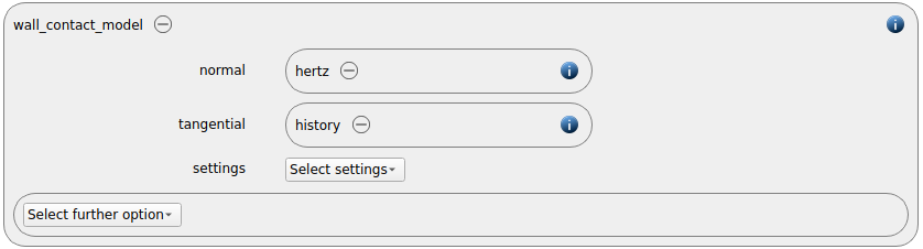
Since we added meshes in the previous section, a wall contact model is also added automatically to this section. We use the default models normal hertz and tangential history:
The powder compression model is activated by adding the powder/update command:

The gravity is enabled automtially:

Per default the gravity has a magnitude of 9.807 and acts into negative z-direction. These defaults can be changed by either setting the magnitude or the direction manually.
Particles
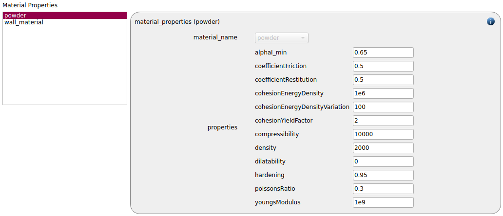
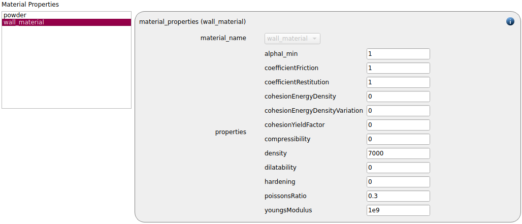
In the general settings tab the material properties for the powder and the wall_material are specified:
powder |
wall_material |
|
Density |
2000 |
7000 |
Young’s modulus |
1e9 |
1e9 |
Poisson’s ratio |
0.3 |
0.3 |
Coefficient of restitution |
0.5 |
1 |
Coefficient of friction |
0.5 |
1 |
Cohesion energy density |
1e6 |
0 |
Cohesion energy density variation |
100 |
0 |
Cohesion yield factor |
2 |
0 |
alphaI_min |
0.65 |
1 |
Compressibility |
10000 |
0 |
Dilatability |
0 |
0 |
Hardening |
0.95 |
0 |
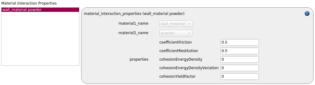
Since two materials are present, also the material interaction properties must be set:
wall_material - powder |
|
Coefficient of friction |
0.5 |
Coefficient of restitution |
0.5 |
Cohesion energy density |
0 |
Cohesion energy density variation |
0 |
Cohesion yield factor |
0 |
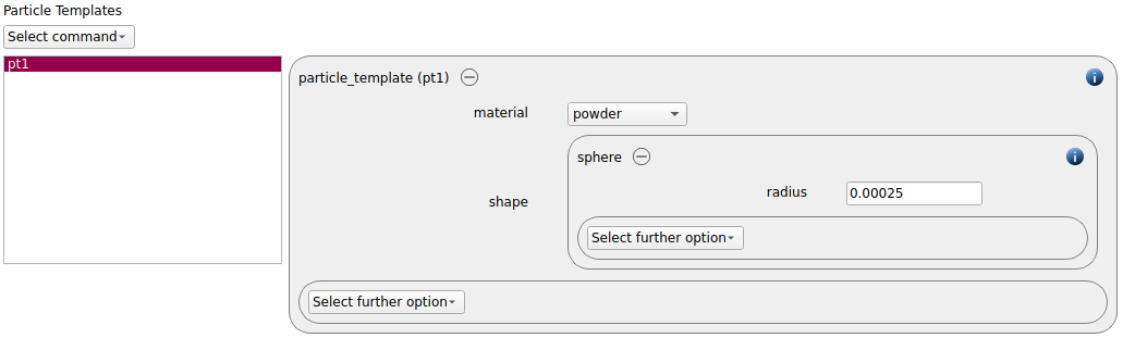
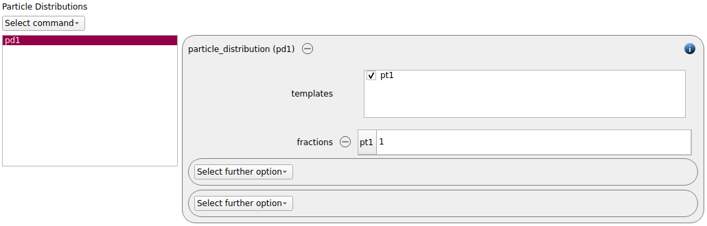
A particle template of shape sphere with radius 0.00025 is added and used for a particle distribution:
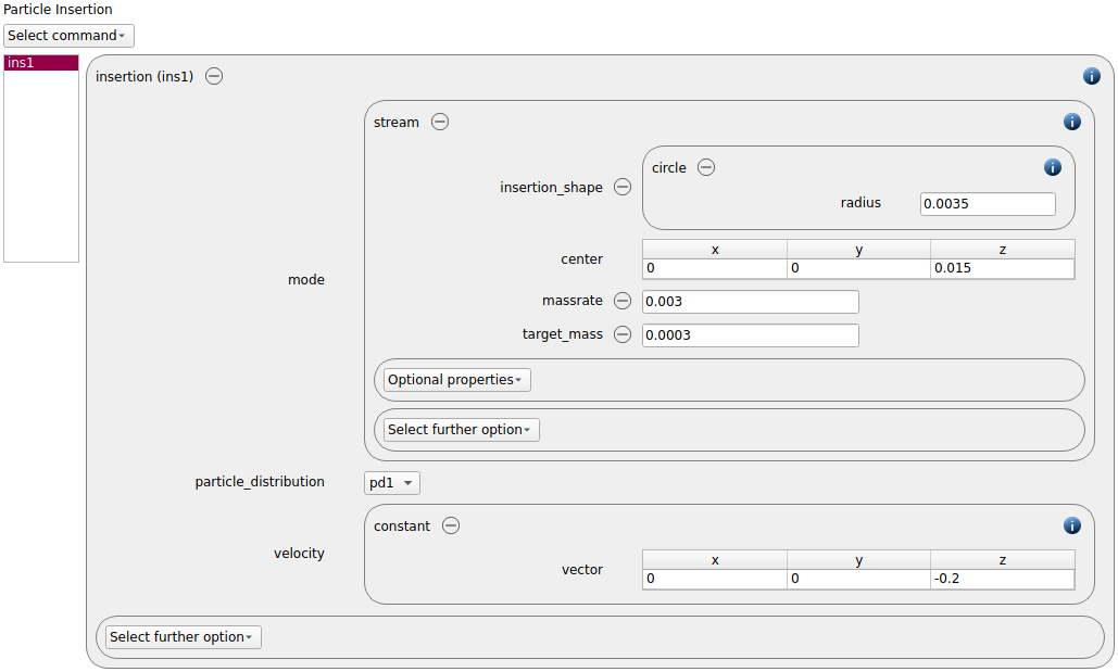
0.0003 kg of particles with a velocity of 0.2 m/s in the negative z-direction is now inserted. We use an insertion command command with mode stream, the massrate is set to 0.003 kg/s. The stream command requires a face for the insertion which can either consist of a mesh or a primitive insertion shape. In our case we are using a circle with a radius of 0.003 m and a center of (0,0,0.015):
Simulation control
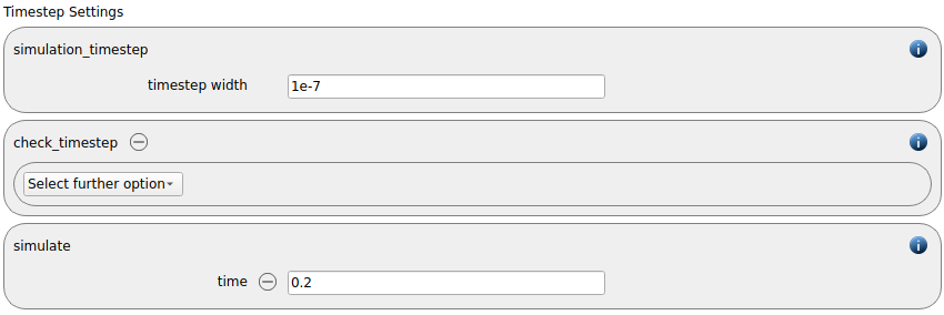
In this tab, we first define the time-step settings such as the desired simulation timestep of 1e-7 seconds and the total simulation time of 0.2 seconds. Per default also the check_timestep command command is enabled, which throws a warning when the time step exceeds 10 % of the Rayleigh or the Hertz time. These thresholds can be changed by setting an alternative value for hertz_fraction or rayleigh_fraction.
Loadbalancing is enabled per default:

Output settings
In this tab we first define the timestep width for the file and the terminal output:
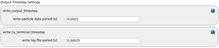
The output_settings command command the takes care that all particle information and the meshes are written to files accordingly. Furthermore it triggers the output of global quantities such as the kinetic energy of the particles or total normal and shear stresses onto meshes to the terminal. Please note that if the output of per-cell information on meshes such as wear, velocity of stress are desired, one has to add the keyword mesh_properties and select the required output. If one or more meshes are added to the meshes list but no mesh properties are selected, all available properties are added to the output.

Running the simulation
After completing the setup and saving it, the simulation can be launched. Change to the Simulation view and set the number of cores to use to 2. Please note that using more cores would rather increase the simulation times instead of decreasing them due to the low number of particles in the simulation. First hit the “Check settings” button, and if the check returns “Check settings successfully completed” the simulation can be run by hitting “Start”.
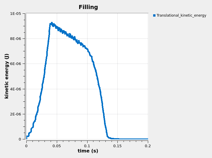
The graph below shows the kinetic energy as a function of time:
Postprocessing with Paraview
After the simulation is completed, all data written with the output_settings command can be visualized automatically by going to the Visualization view and hitting the “Start Paraview” button.
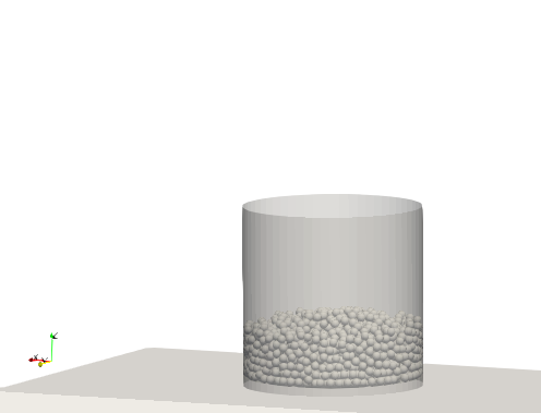
The image below shows the final state of the system:
Case 2: Compression
In this case the lose particle bed is compressed with the help of a servo wall. We start by creating a derived simulation that depends on the filling case.
Meshes and Regions
In the meshes and regions tab we first define a mesh module servo:
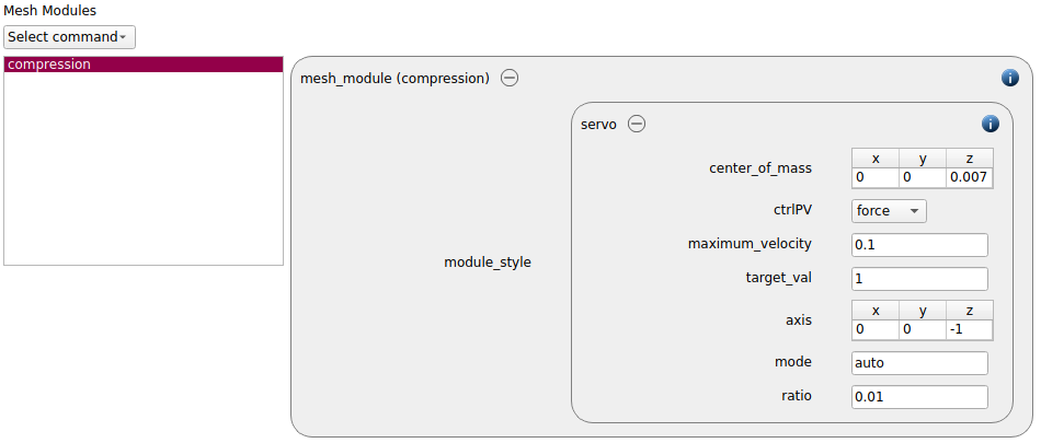
The servo wall will be force controlled with a target value of 1 Newton. We set the maximal velocity of the mesh to 0.1 m/s and for obtaining compression with respect to gravity we set the axis to (0,0,-1). The center of mass is set to (0,0,0.007), the mode is auto and the ratio is set to 0.01.
This mesh module is applied to a mesh:
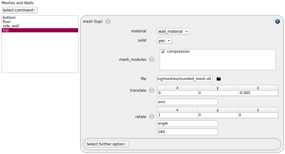
This mesh is based on the same mesh file as the bottom used in the filling simulation, only rotated and translated.
Particles
In the particles tab the insertion command is removed:

Simulation control
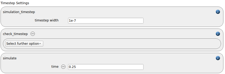
The total simulation time is set to 0.25 seconds:
Running the simulation
After completing the setup and saving it, the simulation can be launched. Change to the Simulation view and launch the simulation. Please make sure that the number of cores is set to 2 there too.
The graphs below shows the z-force on the top wall and its position over time:
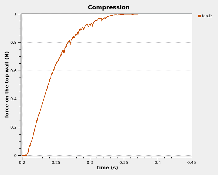
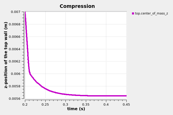
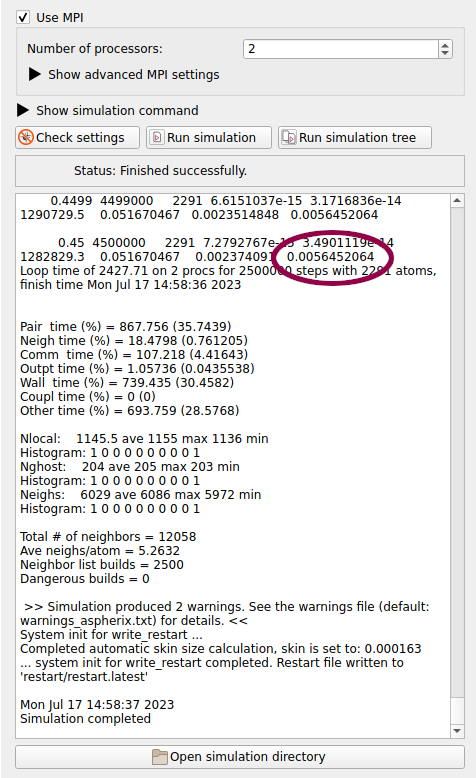
Both values reach a plateau in the course of the simulation time, meaning that the simulation reaches a steady state. We also check the numeric value of the z-position of the wall (here 0.00564… - can be slightly different for different simulation runs). This value will be used in the next simulation, where we will have to select the correct starting position for the proceeding calculation.
Postprocessing with Paraview
After the simulation is completed, all data written with the output_settings command can be visualized automatically by going to the Visualization view and hitting the “Start Paraview” button.
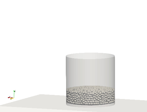
The image below shows the final state of the system:
Case 3: Decompression
In the next simulation we are slowly removing the top wall that compresses the powder and the tablet that has been produced by compressing the powder is moved upwards in the cylinder. An instantaneous removal of the top wall would lead to high forces and potential instabilities, which is why we are using another servo wall command for triggering a smooth upwards motion.
Meshes and Regions
In the meshes and regions tab we rename the existing mesh module servo to decompression and invert the axis to (0,0,1):
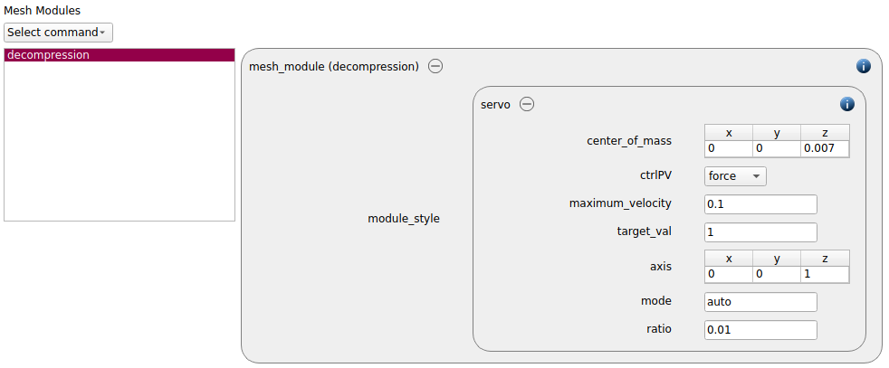
This mesh module remains attached to the top mesh. The top mesh is now translated to the final z-position of the previous calculation (0.0056460860):
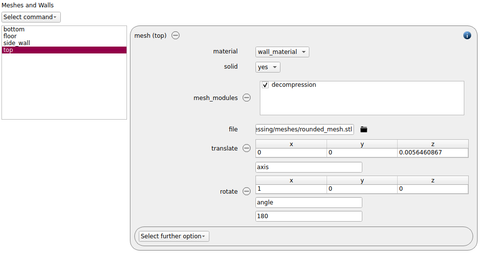
This mesh is based on the same mesh file as the bottom used in the filling simulation, only rotated and translated.
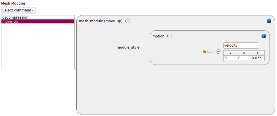
Another mesh module of type motion is created:
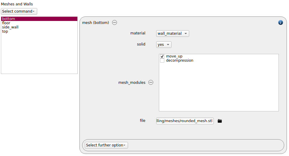
This mesh module is attached to the bottom mesh:
Simulation control
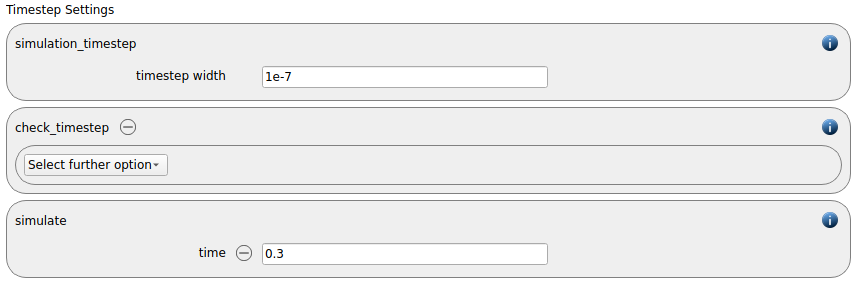
The total simulation time is set to 0.3 seconds:
Custom Settings
Since force and z-position of the top wall are of no increased interest any more, we removed the custom command from the custom settings tab.
Running the simulation
After completing the setup and saving it, the simulation can be launched. Change to the Simulation view and launch the simulation. Please make sure that the number of cores is set to 2 there too.
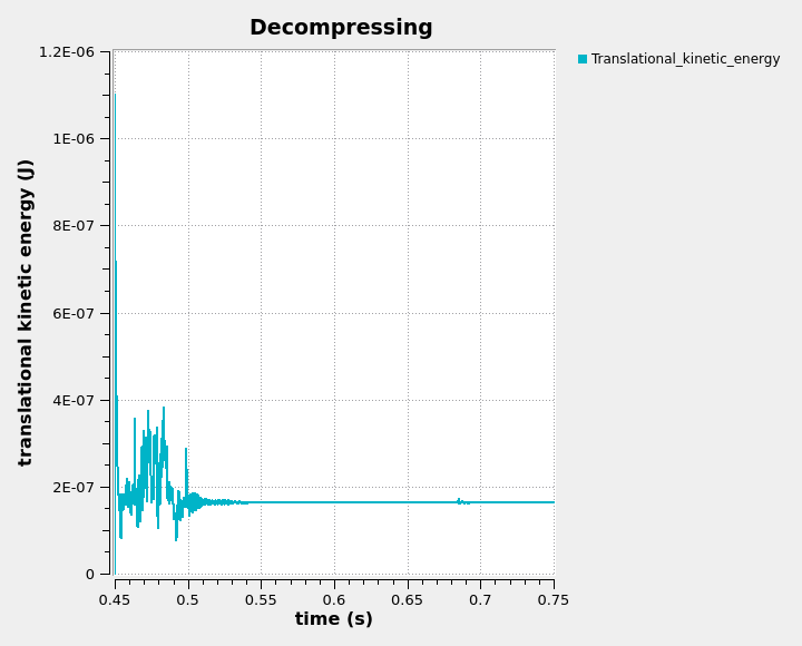
The graphs below shows the kinetic energy over time:
Postprocessing with Paraview
After the simulation is completed, all data written with the output_settings command can be visualized automatically by going to the Visualization view and hitting the “Start Paraview” button.
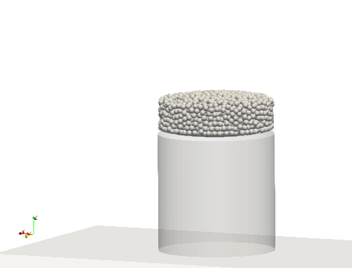
The image below shows the final state of the system:
Case 4: Ejection
In this last simulation the top mesh is entirely removed from the simulation and the tablet is ejected.
Meshes and Regions
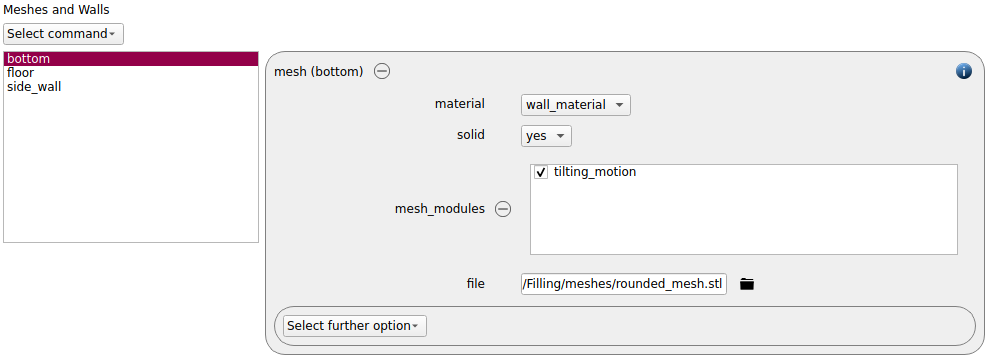
In the meshes and regions tab we removed both the mesh module for the decompression and the top mesh. The mesh module for the motion of the bottom mesh is renamed to tilting_motion and the linear motion is replaced by a rotation:
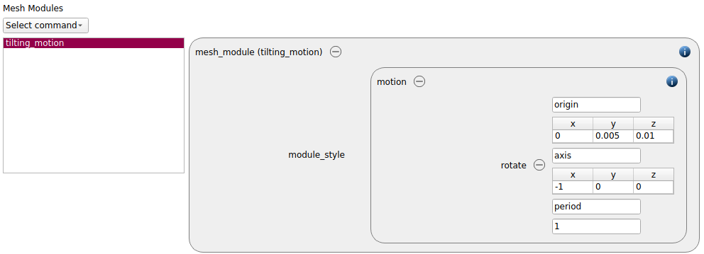
The mesh module is automatically renamed and still attached to the bottom mesh:
Running the simulation
After completing the setup and saving it, the simulation can be launched. Change to the Simulation view and launch the simulation. Please make sure that the number of cores is set to 2 there too.
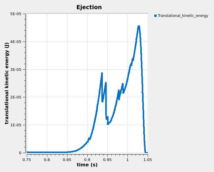
The graphs below shows the kinetic energy over time:
Postprocessing with Paraview
After the simulation is completed, all data written with the output_settings command can be visualized automatically by going to the Visualization view and hitting the “Start Paraview” button.
The image below shows the ejection of the tablet:
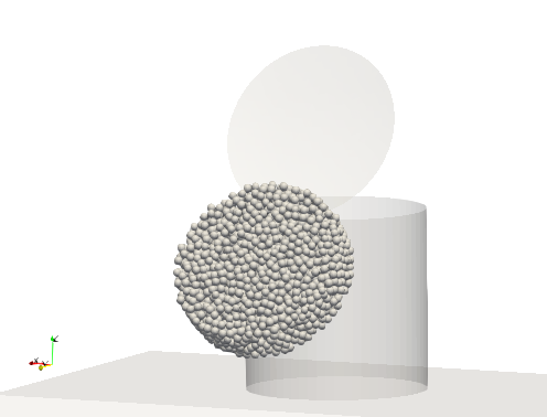
The below image summarizes all four states: