Appification: Spray coating simulation

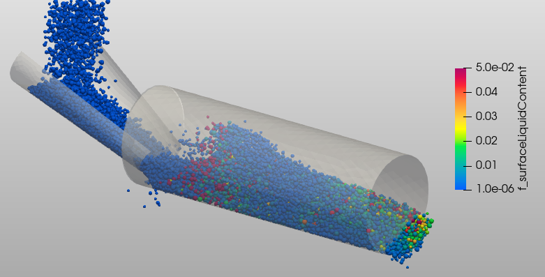
This tutorial consists of two parts: in the first part we show how to set up a simply spray coating case. As shown by the image below we use a chute to insert spherical particles in a rotating drum. In a region at the beginning of the drum liquid is added to the particles on the surface. The rotational motion of the drum leads to a distribution of the liquid among the bulk material.

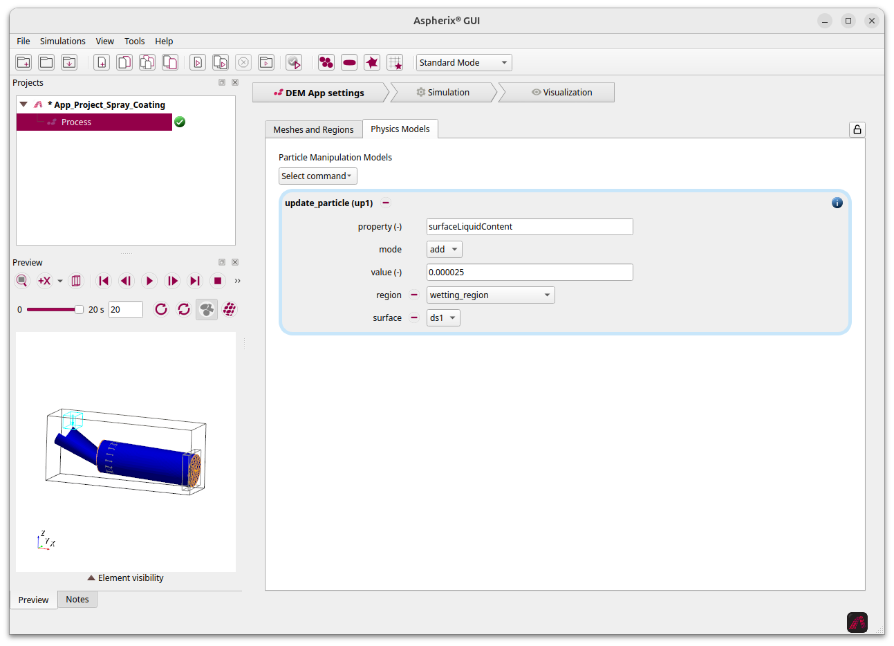
In the second step of the tutorial we show how to transform this full simulation setup to an App in which the user can only modify the rotational velocity of the drum and the amount of liquid that is added to the particles.

Name of the case: App_Project_Spray_Coating

Part 1: Simulation setup

General settings

We start with selecting “sphere” as particle shape:

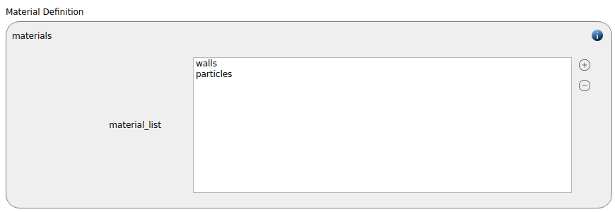
We use two materials command (one for the wall, one for the particles):

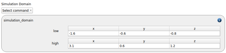
and create a simulation domain that reaches from -1.6 to 3.1 in x-dimension, from -0.6 to 0.6 in y-dimension and from -0.8 to 1.2 in z-dimension:

Meshes and regions

Four different meshes are used in this simulation: a chute that is used for the insertion of the particles, a cylindric mesh that represents the rotating drum and two spherical plates that are used to measure the massflow at the inlet and at the outlet of the drum.

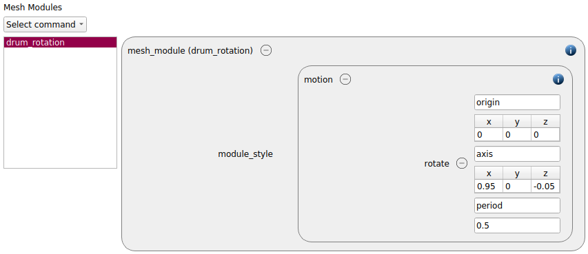
We first start with defining the mesh_module for the rotational motion:

In the next step we load a mesh for the chute:

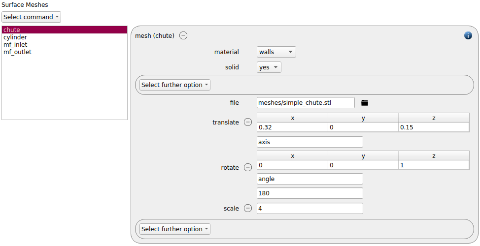
The chute, as well as the cylinder is used as solid and of material “walls”. It is translated by (0.32, 0, 0.15) meters in x, y and z direction and rotated by an angle of 180 degrees around the z axis. Finally a scaling factor of 4 is applied.

Next, the cylindric mesh for the drum is loaded:

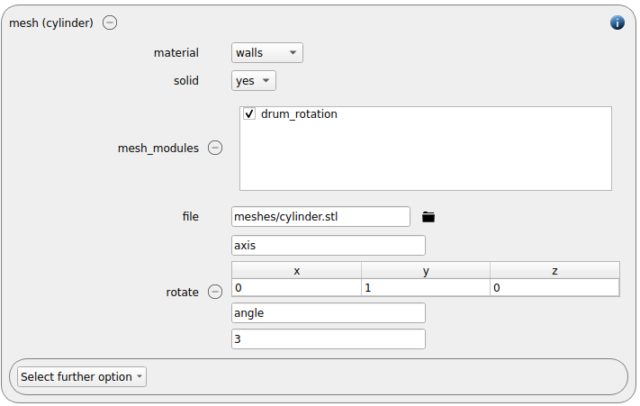
We apply the previously defined motion mesh module to it and rotate it by three degrees around the positive y axis. Together with the rotational motion this slight inclination causes an axial motion of the bulk material.

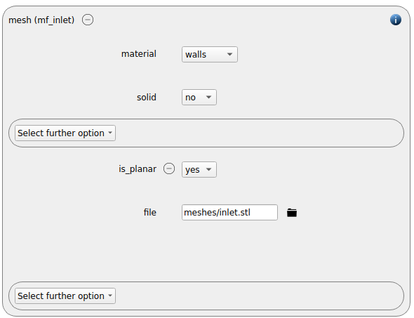
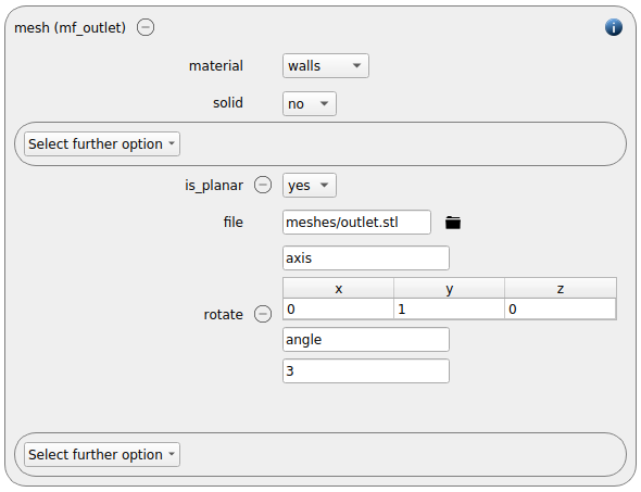
Next, the two meshes for measuring the massflow at the inlet and at the outlet of the drum are added. Please use the configuration “solid no” and “is_planar yes” for both of them. The outlet mesh is rotated by three degrees around the y axis:

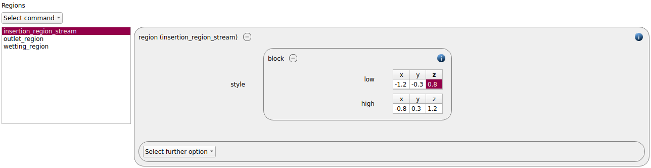
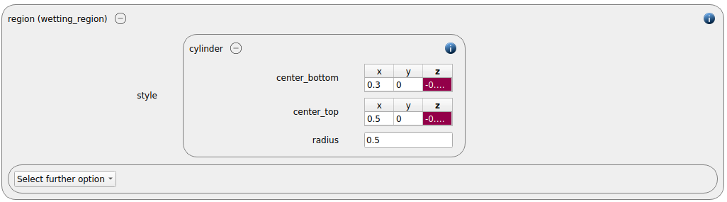
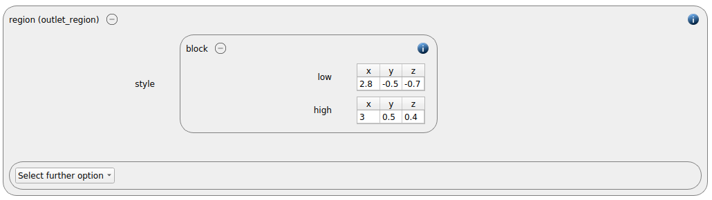
We proceed with defining three different regions: one for the insertion of the particles (above the chute), one region in which the liquid will be applied (at the beginning of the drum) and one region for measuring the average surface liquid content (at the end of the drum):

Physics models

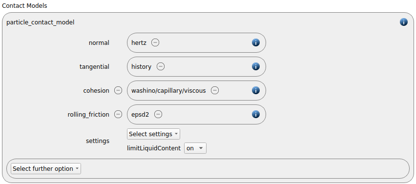
For the particle-particle interactions we use the hertz normal model, the tangential history model and the epsd2 model for the rolling friction. For modelling the liquid bridges between the particles we use the washino/capillary/viscous model:

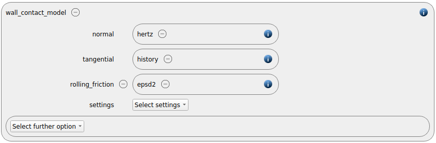
For modelling the particle-wall contacts we use the same models as for that particles except for the cohesion model

The gravity is switched on per default. We use it in the standard configuration (magnitude of 9.807 in negative z-direction), so nothing needs to be changed here:

In the next step we scroll to the bottom of the page and switch on the liquid transport model:

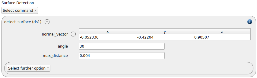
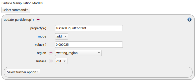
The liquid will be applied using an update_particle command command, and since only surface particles will be affected by the spray, we first apply a detect_surface command command:

Particles

We set the material_properties command for the particles and the walls:

	particles	walls
Density	2500	7000
Young’s modulus	5e6	5e6
Poisson ratio	0.3	0.3
Coefficient of restitution	0.6	1.0
Coefficient of friction	0.5	1.0
Contace angle	70	1.0
Max. liquid content	0.1	1.0
Coefficient of rolling friction	0.01	1.0
Latent heat	0	0
Evaporation temperature	0	0
Liquid heat capacity	0	0

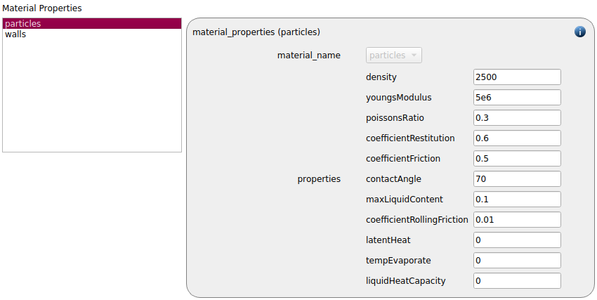
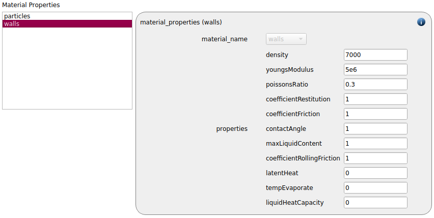
Please note that the latent heat, the evaporation temperature and the liquid heat capacity are not used in this case and that their values will be ignored.

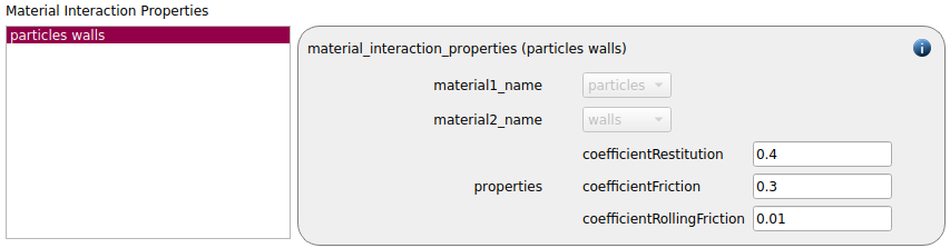
Since two different materials are used, material interaction properties are also defined:

	particles & walls
Coefficient of restitution	0.4
Coefficient of friction	0.3
Coefficient of rolling friction	0.01

The selected physical models also require the definition of several global scalars:

	value
Fluid viscosity	1e-5
Maximal relative separation distance	0.2
Minimal relative separation distance	0.01
Surface liquid content initial	1e-6
Surface tension	10

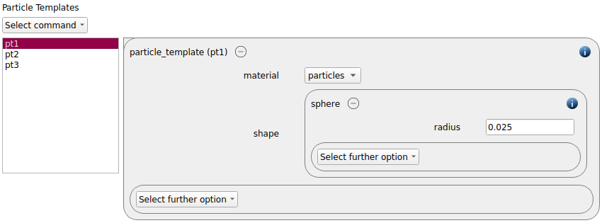
Three particle templates for spheres (radii = 0.015, 0.02 and 0.025) are defined and combined to a particle distribution:

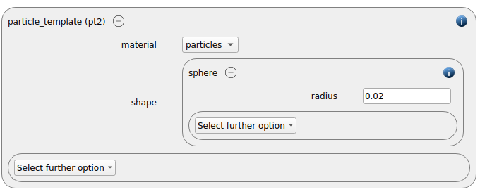
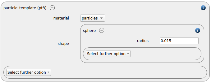
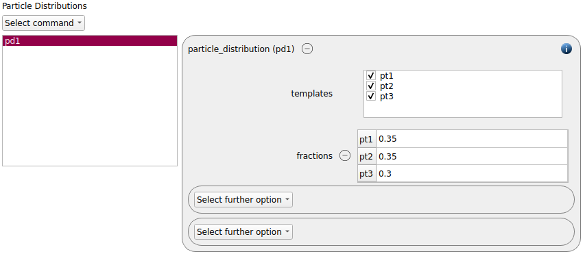
An insertion command command of type rate_in_region is created, which adds material with a massrate of 200 kg/s and a velocity of 1 m/s in negative z-direction. The previously defined insertion region is used:

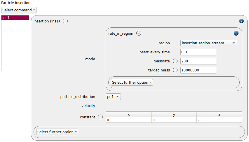
Since we do not want to stop the insertion during the simulation, we define a very high target mass.

Simulation control

In the next section we define the simulation time step and the total simulation time which we set to 20 seconds. Furthermore the check_timestep command command is enabled.

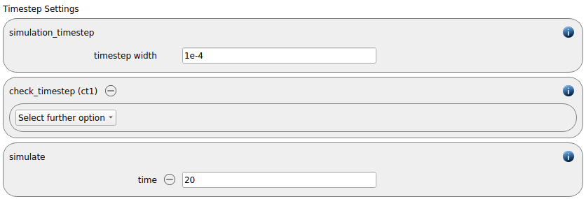
The skin size of the neighbor list command can be calculated automatically, thus we can remove this dummy command.

For an optimal usage of the resources the load balancing is switched on:

Output settings

In this tab we first define the timestep width for the file and the terminal output:

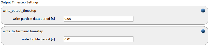
The default output_settings command command is used:

Furthermore, we add two calculate command commands for measuring the massflow at the inlet and outlet of the cylinder:

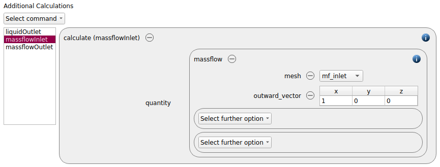
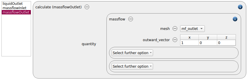
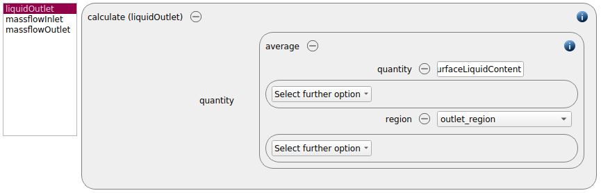
A third calculate command is used to compute the average surface liquid content of the particles in a region towards the end of the cylinder. The quantity can be referenced by id_surfaceLiquidContent:

Simulation and results

Please save the project and change to the Simulation tab. After running the simulation the following curve for the number of particles and the kinetic energy shows:

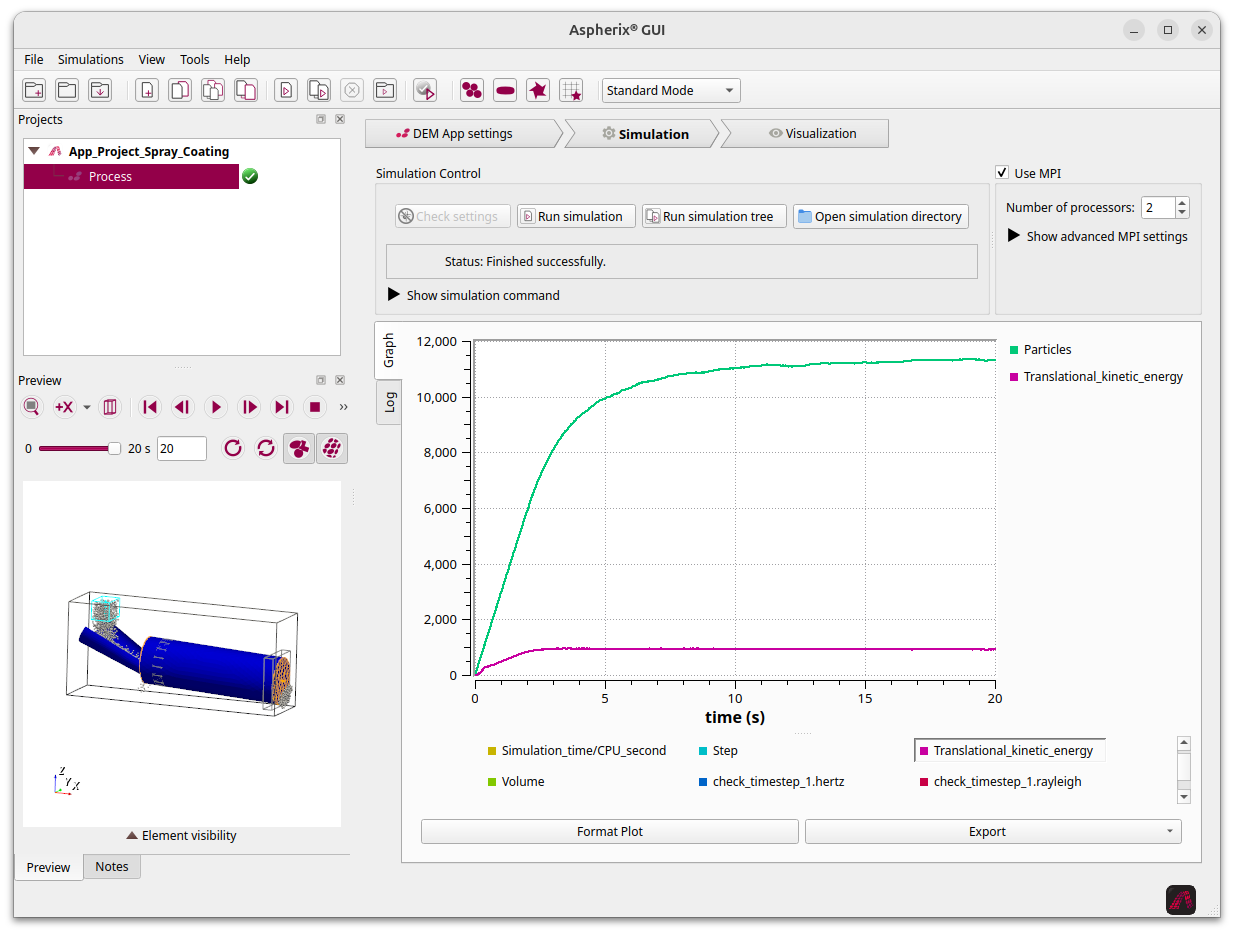
So with respect to these quantities the simulation has reached a steady state.

In addition to that we can also visualize the massflowrate at the inlet and outlet of the drum:

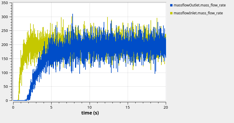
Due to the relatively coarse bulk material and the fine measurement frequency the signal is rather noisy, but it still becomes visible that also the massflow has reached a steady state.

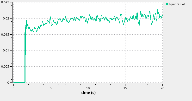
Finally we can also visualize the average surface content of the particles in the outlet region:

The simulation data can be visualized in Paraview (here liquid content of the particles, last time step):

The simulation itself would be completed now. In the next part of this tutorial we want to convert this simulation into an App that only allows the modification of few values and thus makes is clearer and easier to use in production runs.

Part 2: Transforming a simulation to an App

First of all we move back to the DEM Setup window. Then we change from the Standard Mode to the App Creation Mode:

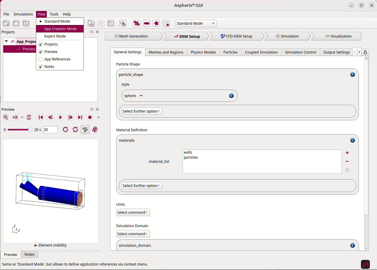
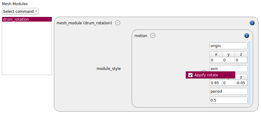
At first glance this does not change much. However, this mode allows us to appify single commands and keywords. Our first target is the rotational motion of the drum. Please go to the Meshes and regions tab, scroll down to the mesh module and right-click the rotation mesh module. This shows a small Window with a check-box called “Appify rotate”. Please check this option:

The second quantity we want to be available in out App is the liquid content that is added. Therefore please move to the Physics models tab and scroll down to the update_particle command. In this case we would like to allow the user to modify the entire command, thus we right-click on the command name itself and check the “Appify update_particle” box:

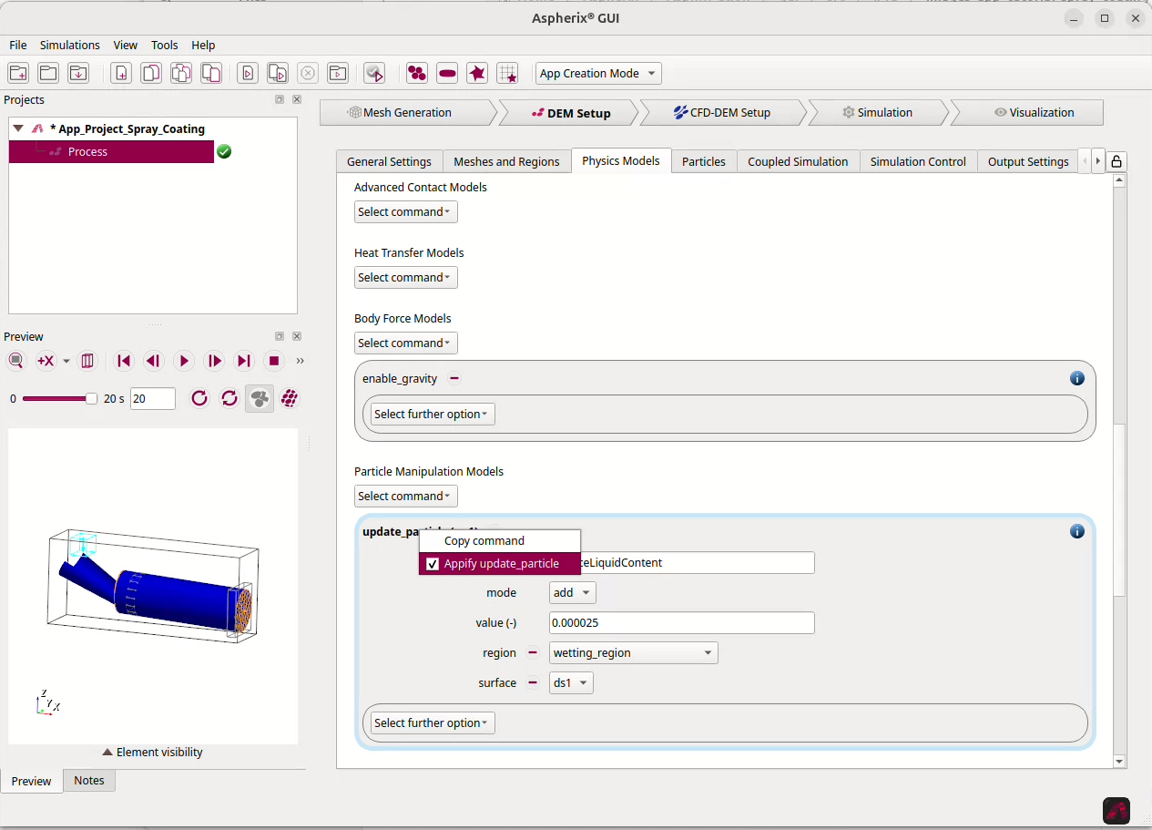
Appified commands receive a light-blue frame whereas appified keywords are marked by a light blue column on the right hand side.

After these two simple steps the Appification is completed. We save the project and switch back to the Standard Mode. We now see the visualization of or newly created app. The DEM Setup section is now replaced by a DEM App settings section that only contains those quantities that were marked for modification:

Whenever a user opens a new Aspherix® GUI and loads a project with an appified simulation it gets visualized like that. The full simulation setup is then only visible in the App Creation Mode or in the Expert Mode.

For more details on appification please see this section of the documentation.