LaEuScalarTemp

Syntax

Defined in couplingProperties dictionary.

forceModels
(
    LaEuScalarTemp
);
LaEuScalarTempProps
{
    velFieldName         "U";
    tempFieldName        "T";
    voidfractionFieldName "voidfraction";
    EuFieldName          word;
    compressible         switch;
    lambda               scalar;
    Cp                   scalar;
    TInterpolationType   word;
    maxSource            scalar;
    temperatureBlendFactor scalar;
    automaticBlending    switch;
    NuCorrelation        "LiMason";
    useImplicitCFDSource switch;
    useImplicitDEMSource switch;
    lambdaEvaporationCorr switch;
    lambdaEvaporationCorr_Bird switch;

    // (optional) forceSubModel switches
    verbose              switch;
    interpolation        switch;
    scalarViscosity      switch;
    scaleDrag            scalar;
    scaleDH              scalar;
};

velFieldName = name of the finite volume fluid velocity field (default: “U”)
tempFieldName = name of the finite volume scalar temperature field (defaut: “T”)
voidfractionFieldName = name of the finite volume voidfraction field (default: “voidfraction”)
EuFieldName = name of the finite volume field used for calculating the fluid-particle heat transfer (default: TSource if compressible false or QSource if compressible true)
compressible = enable correct fluid-particle heat transfer when using a compressible solver. cfdemSolverChem, cfdemSolverRhoPimple, and cfdemSolverInter are automatically detected as compressbile solvers. For all other solvers, this setting is false by default.
lambda = fluid thermal conductivity [ $W/(m K)$ ]. If chosen less than zero, then the thermal conductivity field is derived automatically from the thermophysical properties defined in the thermophysicalProperties file. This is possible only if the solver uses the thermophysical model library, like for example cfdemSolverChem (default: -1).
Cp = specific heat capacity of fluid [ $J/(kg K)$ ]. (default: -1)

Note

If set to values below zero (or kept at default), the thermal conductivity field is derived automatically from the thermophysical properties defined in the thermophysicalProperties file. This works only if the solver uses the thermophysical model library, like for instance cfdemSolverChem. In general, thermophysicalProperties are used for compressible fluids.

Note

Cp is only read if this model operates on an incompressible fluid in standalone mode. If run with cfdemSolverPimple, Cp is read from the scalarTransportProperties dictionary.
maxSource = maximum value of the heat flux (in absolute value) imposed on a CFD cell (default: 1e30)
temperatureBlendFactor = limit fluid-particle heat transfer on both CFD and DEM side (default: 0, i.e. no blending)
automaticBlending = automatically determine if blending should occur (default: false)
NuCorrelation = chooses the heat correlation to be used for Nusselt number calculation. Valid options: “LiMason”, “Deen” and “Gunn” (default: “LiMason”)
useImplicitCFDSource = use an implicit source term for particle-fluid heat transfer in the temperature or heat equation. (default: true)
useImplicitDEMSource = use an implicit source term for particle-fluid heat transfer in DEM. (default: true, matching the default in DEM)
lambdaEvaporationCorr = correct the fluid thermal conductivity at the particle for evaporation effects (default: false)
lambdaEvaporationCorr_Bird = correct the fluid thermal conductivity at the particle for evaporation and composition effects. See details below. This setting is mutually exclusive with lambdaEvaporationCorr yes. (default: false)
tempEvaporation = model parameter for lambdaEvaporationCorr_Bird (default: 373.)
tempBase = model parameter for lambdaEvaporationCorr_Bird (default: 293.)
correctionFactor = model parameter for lambdaEvaporationCorr_Bird (default: 2.)
correctionFuncExp = model parameter for lambdaEvaporationCorr_Bird (default: 2.)

This forceModel reads the following forceSubModel switches and overwrites the defaults as indicated in parentheses:

scaleDrag
scaleDH
verbose
interpolation (default: true)
scalarViscosity

Examples

When using a compressible solver, e.g. cfdemSolverChem, the following settings should be used.

forceModels
(
    LaEuScalarTemp
);
LaEuScalarTempProps
{
}

When using an incompressible solver, e.g. cfdemSolverPiso, the following settings should be used.

forceModels
(
    LaEuScalarTemp
);
LaEuScalarTempProps
{
    lambda                   0.024;
    Cp                       1000.0;
}

Description

The model calculates the convective heat flux between particles and fluid. Three possible relations can be used for calculating the Nusselt number as a function of Reynolds and Prandtl number as well as the voidfraction $\alpha$ , namely the ones from Li and Mason, Deen et al. or Gunn:

LiMason

$\mathit{Nu} = \left\{ \begin{array}{ll} 2 + 0.6 \mathit{\alpha}^{3.5} \sqrt{Re} \mathit{Pr}^{1/3}, & \text{if}\ \mathit{Re} < 200 \\ 2 + \left( 0.5 \sqrt{Re} + 0.02 Re^{0.8} \right) \mathit{\alpha}^{3.5} Pr^{1/3}, & \text{if}\ 200 <= \mathit{Re} < 1500 \\ 2 + 0.000045 \mathit{\alpha}^{3.5} \mathit{Re}^{1.8}, & \text{else} \end{array} \right.$
Deen

$\mathit{Nu} = \left( 7 - 10 \mathit{\alpha} + 5 \mathit{\alpha}^2 \right) \left( 1 + 0.17 \mathit{Re}^{0.2} \right) \mathit{Pr}^{1/3} + \left( 1.33 - 2.31 \mathit{\alpha} + 1.16 \mathit{\alpha}^2 \right) \mathit{Re}^{0.7} \mathit{Pr}^{1/3}$
Gunn

$\mathit{Nu} = \left( 7 - 10 \mathit{\alpha} + 5 \mathit{\alpha}^2 \right) \left( 1 + 0.7 \mathit{Re}^{0.2} \right) \mathit{Pr}^{1/3} + \left( 1.33 - 2.4 \mathit{\alpha} + 1.2 \mathit{\alpha}^2 \right) \mathit{Re}^{0.7} \mathit{Pr}^{1/3}$

The user needs to specify the thermal conductivity and specific heat capacity of the fluid, if these properties are not already read from the thermophysicalProperties file. In case the solver reads this file and, at the same time, the user specifies values for Cp and lambda in couplingProperties/LaEuScalarTempProps that are larger than zero, then the model will use the latter ones to calculate the heat flux.

If using this model with a compressible solver, the flag compressible is set to true automatically. In any case it needs to be set to true when using a compressible solver to will ensure the conservation of energy in the system.

If verbose true, the model will also write the fields used for Cp and lambda.

The setting temperatureBlendFactor sets a blending factor $\alpha_\mathrm{blend}$ which taps into the calculation of fluid-particle heat transfer by changing the fluid temperature. The fluid temperature is blended to the current thermal equilibrium:

$T_\mathrm{HT} = (1 - \alpha_\mathrm{blend}) T_\mathrm{fluid} + \alpha_\mathrm{blend} T_\mathrm{eq}$

$T_\mathrm{eq} = \frac{ m_\mathrm{part} C_\mathrm{p,part} T_\mathrm{part} + m_\mathrm{fluid} C_\mathrm{p,fluid} T_\mathrm{fluid} } { m_\mathrm{part} C_\mathrm{p,part} + m_\mathrm{fluid} C_\mathrm{p,fluid} }$

Note

To set particle density and heat capacity, this model requires the additional user input particleRho and particleCp. Both are scalar lists that need to provide the particle material density and heat capacity in the same order as set on the DEM side.

The setting automaticBlending allows the model to automatically determine whether temperature blending should be applied. The blending factor is then determined on a per-particle basis if the CFD timestep $\Delta{t}_\mathrm{CFD}$ is greater the the critical parcel-fluid heat-exchange timestep $\Delta{t}_\mathrm{crit,HE}$ :

$\Delta{t}_{crit,HE} = \left(\frac{m_\mathrm{fluid,cell} C_\mathrm{p,fluid}}{m_\mathrm{parcel} C_\mathrm{p,particle}}\right) \tau_\mathrm{p,HE}$

$\tau_\mathrm{particle,HE} = \frac{d_\mathrm{particle} \rho_\mathrm{particle} C_\mathrm{p,particle}}{6 \alpha_\mathrm{HE}}$

The automatic blending feature takes coarse-graining into account during the scaling of the particle’s heat transfer timescale $\tau_\mathrm{particle,HE}$ .

In case the particles contain evaporating liquid, the fluid thermal conductivity can be corrected using conductivity_evaporation_correction yes:

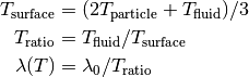
$T_\mathrm{surface} &= (2 T_\mathrm{particle} + T_\mathrm{fluid}) / 3 \\ T_\mathrm{ratio} &= T_\mathrm{fluid} / T_\mathrm{surface} \\ \lambda(T) &= \lambda_0 / T_\mathrm{ratio}$

Alternatively an approximation of the Bird correction is available with conductivity_evaporation_correction_Bird yes:

$\lambda(T) = \lambda_0 (f - 1) \left( \frac{T - T_b}{T_e - T_b} \right)^e + \lambda_0$

with

$\lambda_0$ : the fluid thermal conductivity in the cell (e.g. set by keyword lambda)
$T_e$ : the liquid evaporation temperature as specified by the tempEvaporation keyword
$T_b$ : the model function base temperature set using the tempBase keyword
$f$ : the factor of fluid thermal conductivity at evaporation temperature, i.e. $f = \frac{\lambda(T_e)}{\lambda_0}$ , specified by the correctionFactor keyword
$e$ : the model function exponent set using the correctionFuncExp keyword

The exponent must not be negative and the expression is limited to values in the interval $[T_b, T_e]$

Note

conductivity_evaporation_correction yes and conductivity_evaporation_correction_Bird yes are mutually exclusive.

Restrictions

Works only with solvers which solve an energy equation and provide the necessary TSource or QSource field, either natively or via STM model, e.g. cfdemSolverChem, cfdemSolverPimple, cfdemSolverRhoPimple.

Literature

[1] Li, J., Mason, D. J. A computational investigation of transient heat transfer in pneumatic transport of granular particles. Powder Technology 112.3 (2000) 273-282.

[2] Deen, N. G., et al. Review of direct numerical simulation of fluid–particle mass, momentum and heat transfer in dense gas–solid flows. Chemical Engineering Science 116 (2014) 710-724.

[3] Gunn, D. J. Transfer of heat or mass to particles in fixed and fluidised beds. International Journal of Heat and Mass Transfer 21.4 (1978) 467-476.