cohesion model liquidbridge/general

Syntax

cohesion liquidbridge/general [other model_type/model_name pairs as described here ] settings keyword values

two mandatory keyword/value pairs need to be appended after the keyword settings (after all models are specified)

normal_model values = 'adams_perchard' or 'pitois' or 'washino' or 'washino_powerlaw'
tangential_model values = 'goldman' or 'xu' or 'washino' or 'xu_powerlaw'

zero or more keyword/value pairs may be appended after the keyword settings (after all models are specified)

limitLiquidContent values = 'on' or 'off'
  on = enables the model parameter maxLiquidContent
  off = standard implementation without a limiter for the per particle liquid content
modifyLbVolume values = 'on' or 'off'
  on = enables the model parameter lbVolumeFraction
  off = standard implementation with lbVolumeFraction = 0.05

Associated material properties

Material properties

contactAngle ( $\theta$ ): contact angle between particle’s material and liquid [deg]
maxLiquidContent ( $\gamma_{l,max}$ ): maximum liquid content of a particle of this material. It is expressed as fraction of the particle’s volume [ $\cdot; [0, 1]$ ] (required only if limitLiquidContent on)
minLiquidLayerThickness: the minimal thickness of the liquid film (default: 0)

Global scalars 

minRelativeSeparationDistance ( $d_{min}$ ): ratio between the minimum distance between particles’ surface and the effective radius $r^*$ . For surface separations below this value, the liquid bridge model assumes a distance equal to $d_{min} r^*$ [ $\cdot; ]0, \cdot]$ ]
maxRelativeSeparationDistance ( $d_{max}$ ): ratio between the maximum distance between particles’ surface and the effective radius $r^*$ at which the liquid bridge can exists [ $\cdot; ]0, \cdot]$ ]
surfaceLiquidContentInitial ( $\gamma_{l,0}$ ): particle initial liquid content. It is expressed as fraction of the particle’s volume [ $\cdot; [0, 1]$ ]
fluidViscosity
- ( $\mu$ ) dynamic viscosity of the liquid if fluidPowerLawExponent not given or equal to one (fluid is considered Newtonian) [pressure*time; $[0,\cdot]$ ]
- ( $K$ ) flow consistency of the liquid if fluidPowerLawExponent is $\neq 0$ [pressure*time^n; $[0, \cdot]$ ]
surfaceTension ( $\sigma$ ): surface tension of the liquid [force/length; $[0, \cdot]$ ]
lbVolumeFraction ( $\gamma_b$ ): liquid amount forming the liquid bridge. It is expressed as fraction of the total liquid contained by the two particles forming the bridge [ $\cdot; [0, 1]$ ] (required only if modifyLbVolume on)
fluidPowerLawExponent ( $n$ ): power index [ $\cdot; [0, \cdot]$ ]
liquidRedistributionFactor: ( $\phi$ ) multiplicative factor for particle redistribution upon bridge breaking (default: 1) [ $- ; [0,1]$ ]

Description

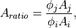
This model adds viscous and capillary forces due to a liquid bridge between two particles. When two particles are close enough, a bridge is formed, which breaks again once the particles are separated. When the bridge breaks, it is assumed that the surface liquid volume distributes evenly to the two particles by default. This behavior can be adjusted by setting the material property liquidRedistributionFactor ( $\phi$ ). The liquid forming the bridge is distributed according to the area ratio of the particles involved in the contact where each area is adjusted by this property, i.e. the ratio is given as:

$A_{ratio} = \frac{\phi_j A_j}{\phi_i A_i},$

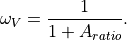
and the volume weight is then

$\omega_V = \frac{1}{1 + A_{ratio}}.$

Different force models for normal and tangential interaction via Newtonian or power-law fluids can be chosen.

The model parameter maxLiquidContent allows to limit the maximum liquid content per-particle (enabled by the keyword limitLiquidContent). In case this feature is enabled, the maxRelativeSeparationDistance will be overwritten to allow the maximum volume to be achieved. The model parameter surfaceLiquidContentInitial is the initial liquid content of the particles as fraction of their volume.

If this contact model is used for mesh walls, they will need to have an associated mesh module liquidtransfer.

If modifyLbVolume on, it is possible to define the amount of liquid that forms each liquid bridge via the model parameter lbVolumeFraction. For modifyLbVolume off, lbVolumeFraction is set by default to 0.05.

The minimum and maximum separation distance ratios control the distance range in which the model is active. Liquid bridges are always considered to rupture at a distance of $r^* d_{max}$ . The value for minRelativeSeparationDistance is used to avoid divergence of the force models. For surface separations below this value, the distance is assumed to be $r^* d_{min}$ .

Force computation

The normal models adams_perchard, pitois and washino are all Newtonian models for interstitial fluids and are described in Washino et al. [1]. Adams-Perchard is a pure lubrication model that does not take into account the finite size of a liquid bridge, while the Pitois and Washino model take the finite extent of the liquid bridge into account. The normal model washino_powerlaw from Washino et al. [3] computes the normal force due to a liquid bridge formed by a power-law fluid.

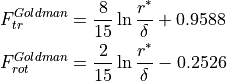
The tangential models goldman, xu and washino, described in Washino et al. [2], consider Newtonian fluids. Again, the Goldman model is actually a lubrication model that does not take into account the finite size of a liquid bridge, while the Xu and Washino models consider a finite liquid bridge. The xu_powerlaw model computes the tangential force for a liquid bridge formed by a power-law fluid, see Xu et al. [4]. For the Xu model, the force only depends on the tangential relative velocity, while the Goldman and Washino models additionally compute a force/torque due to relative angular velocity of the particles.

The models for Newtonian fluids can be combined freely. The power-law models require each other. Please beware when using power-law models, a lower timestep might be required to discretize the non-linear behavior.

In a power-law fluid, the viscosity is given by

$\mu = K \dot{\gamma}^{n-1}$

where $K$ is the flow consistency (set via fluidViscosity), $\dot{\gamma}$ is the shear rate, and $n$ is the power index of the fluid, set via fluidPowerLawExponent

In addition to the viscous force models, a capillary force as in Rabinovich et al. acts between the particles.

In the following, detailed description of the force computation, the following quantities are used:

symbol	meaning
$r_{ij}$	radius of particle $i$ , $j$
$\delta$	minimal width of gap between particles
$V_{lb}$	volume of the liquid bridge
$a$	width of the liquid bridge at particle surface
$H(a)$	width of gap between particles at liquid bridge width

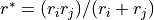
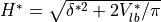
Forces are computed in dimensionless form, thus the following quantities are introduced:

name	equation
effective radius	$r^* = (r_i r_j)/(r_i + r_j)$
reduced surface separation	$\delta^* = \delta / r^*$
reduced liquid bridge volume	$V_{lb}^* = V_{lb} / r^{*3}$
reduced liquid bridge width	$a^* = a / r^*$
reduced gap width at $a^*$	$H^* = \sqrt{\delta^{2} + 2 V_{lb}^/\pi}$

Normal Models

All equations for normal forces for Newtonian fluids are taken from Washino et al. [1]. All three normal force models follow the scheme

$F_n = \frac{3}{2} \mu r^* v_n \times F_n^{model}$

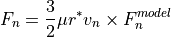
with

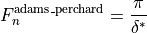
$F_n^{\mathrm{adams\_perchard}} = \frac{\pi}{\delta^*}$

for the adams_perchard model,

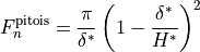
$F_n^{\mathrm{pitois}} = \frac{\pi}{\delta^*} \left( 1 - \frac{\delta^*}{H^*} \right)^2 \\$

for the pitois model , and

$\begin{align*} A & = 0.72 \delta^{*4} + 1.8 \delta^{*3} \\ B & = -\delta^{*4} + 2.5 \delta^{*3} - 2.4 \delta^{*2} \\ F_n^{\mathrm{washino}} & = \frac{\pi}{\delta^*} \left[ \left( 1-\frac{\delta^*}{H^*} \right)^2 + \frac{A}{\delta^*} \left( \frac{1}{\delta^*} - \frac{1}{H^*} \right) + \frac{B}{\delta^*} \left( H^* - \delta^* \right) \right] \end{align*}$

for the washino model.

The washino_powerlaw model (Washino et al. [3]) computes the normal force for a liquid bridge formed by a power-law fluid. The model is based on work by Lian et al. [6] and Xu et al. [4]. According to Xu et al., this force can be expressed as

$\begin{align*} R_{lb} & = \left[ -2 r^* \delta + 2 \left( r^{*2} \delta^2 + \frac{r^* V_{lb}}{\pi} \right)^{1/2} \right]^{1/2} \\ c & = \frac{R_{lb}^2}{2 r^* \delta} \\ F_n & = 2 \pi \left( \frac{2n+1}{n} \right)^n \frac{R_{lb}^{n+3}}{\delta^{2n+1}} K (v_n)^n \times f_n(n, c) \\ \end{align*}$

with $f_n(n, c)$ the dimensionless normal force. According to Lian et al. [6], this dimensionless force can be expressed as

$\begin{align*} f_{Lian} (n, c) & = \left( \frac{1}{2c} \right)^{(n+3)/2} \left[ f_1(n) + f_2(n, c) \right] \\ f_1(n) & \approx 3 \exp{(-2.40 n)} + 1.5 \exp{(-1.06n)} \\ f_2 (n, c) & = \begin{cases} 2^{5/3} \left[ \ln{ \left( \frac{\left(2c\right)^{1/2}}{4} \right) } + \frac{5}{3} \left( \frac{1}{2c} \frac{1}{16} \right) \right] & n = 1/3 \\ 2^{2n+1} \left[ \frac{\left(2c\right)^{(1-3n)/2} - 4^{1-3n}}{1-3n} + \frac{4n+2}{3n+1} \left( \frac{1}{\left(2c\right)^{(1+3n)/2}} - \frac{1}{4^{1+3n}} \right) \right] & n \neq 1/3 \end{cases} \end{align*}$

This model yields good results for $c > 8$ , but diverges for $c \rightarrow 0$ . Thus, Washino et al. [3] added the following correction:

$\begin{align*} N & = \begin{cases} 2n+1 & \text{for } n < 1/3 \\ \frac{n+3}{2} & \text{for } n \geq 1/3 \end{cases} \\ \Omega & = \frac{\left[ \frac{1}{(n+3) f_{Lian}(n,c)} \right]^{1/N} - 1}{8} \\ f_{washino\_powerlaw} (n,c) & = \begin{cases} \frac{1}{n+3} \left( \frac{1}{1 + \Omega c} \right)^N & \text{for } c < 8 \\ f_{Lian}(n,c) & \text{for } c \geq 8 \end{cases} \end{align*}$

Tangential Models

Force computation for tangential forces is split up in translational and rotational components.

For Newtonian fluids, all equations are taken from Washino et al. [2]. The general form of the tangential force reads

$F_t = -6 \pi \mu r^* \left( U F_{tr} - r^* \omega F_{rot} \right)$

with $U$ being the relative tangential velocity, and $\omega$ the relative angular velocity of the two particles. The force equations for the individual models are listed below:

For the goldman model, the force equations read

$\begin{align*} F_{tr}^{Goldman} & = \frac{8}{15} \ln{\frac{r^*}{\delta}} + 0.9588 \\ F_{rot}^{Goldman} & = \frac{2}{15} \ln{\frac{r^*}{\delta}} - 0.2526 \\ \end{align*}$

In the xu model, only translational tangential force is considered:

$\begin{align*} \lambda & = 2 r^* / \max{(r_i, r_j)} \\ c & = \frac{B^2}{2 r^* \delta} \\ F_{tr}^{Xu} & = \frac{2 + 3 \lambda}{15} \ln{\left(1+c\right)} + \frac{ \left(\ \lambda-1 \right) \left(\ \lambda-2 \right)}{5} \left[ \ln{\left(1+c\right)} - \frac{1}{1+c} \right] \\ F_{rot}^{Xu} & = 0 \\ \end{align*}$

Note: the $B$ in the Xu model is not the same $B$ as in the normal Washino model!

The washino model can be expressed as

$\begin{align*} \gamma & = 0.076 \\ A_T & = \left[ \frac{\lambda-1}{10} + \left( \frac{\lambda-1}{8} - \frac{\lambda-1}{10} \right) \exp{\left( -\gamma c \right)} \right] \frac{1}{1+c} \\ A_R & = \left[ \frac{1}{10} + \left( \frac{-1}{8} - \frac{-1}{10} \right) \exp{\left( -\gamma c \right)} \right] \frac{1}{1+c} \\ F_{tr}^{Washino} & = 4 A_T c \left( 1-\lambda \right) + \left[ 2 A_T c \left( \lambda-1 \right) + 4 A_T \left( \lambda-1 \right) + \frac{1}{3} \right] \ln{\left(1+c\right)} \\ \end{align*}$

$F_{rot}^{Washino} & = 4 A_R c \left( 1-\lambda \right) + \left[ 2 A_R c \left( \lambda-1 \right) + 4 A_R \left( \lambda-1 \right) + \frac{1}{3} \right] \ln{\left(1+c\right)} \\$

In the xu_powerlaw model, the tangential force is expressed as

$F_{tr}^{xu\_powerlaw} & = 2 \pi c \delta^{1-n} K r^* (v_n)^n \times f_{tr}^{xu\_powerlaw}$

with the dimensionless force

$f_{tr}^{xu\_powerlaw} = \frac{n^2 + 3n + 3 \lambda - 2}{c(n-1)(n^2+3n+1)} \left[ 1 - \frac{1}{(1+c)^n} \right] + \frac{3 (\lambda-1) (n \lambda - n - 1)}{cn (n-1) (n^2 + 3n + 1)} \left[ 1 - \frac{1 + cn}{(1+c)^n} \right]$

with $\lambda$ as above in the xu tangential model and $c$ as defined in the washino_powerlaw normal model.

Just as in the xu model for Newtonian fluids, no rotational tangential force is considered in the xu_powerlaw model.

Capillary force

In addition to the models chosen by the user, a capillary force as in Rabinovich et al. acts between the particles. This force can be expressed as

$\begin{align*} C & = \left[ -1 + \sqrt{ 1 + 2 V_{lb} / \pi r^* \delta^2} \right] \\ d \left(\delta, V_{lb} \right) & = \frac{\delta}{2} C \\ \alpha & = \sin \left( \frac{\delta}{r^*} C \right) \\ F \left( \delta, V_{lb} \right) & = \frac{2 \pi r^* \gamma^* \cos \sigma}{1 + \left( \delta / 2 d \left(\delta, V_{lb} \right) \right)} - 2 \pi r^* \sin \alpha \sin \left(\sigma+\alpha\right) \\ \end{align*}$

where $\sigma$ is the surface tension of the fluid. $\gamma^* = (\gamma_i+\gamma_j)/2$ is used as effective contact angle, where $\gamma_{ij}$ are the individual contact angle values for particles $i$ , $j$ .

Liquid transport

By default, this model automatically instantiates a scalar transport equation that solves for the surface liquid content of each particles, expressed in volume percentage of solid volume, i.e., $4/3 \pi r^3$ . The surface liquid volume is assumed to be small, i.e. it is assumed to have no effect on the particle mass, diameter and density.

The user can override the default behavior by explicitly specifying a fix that solves for the surface liquid transport between particles. Such fixes are fix liquidtransport/porous or fix liquidtransport/sponge

Minimum thickness of liquid film

If minLiquidLayerThickness is set to a value larger than 0, the liquid film covers the particle completely only if the resulting liquid film thickness is larger than the value set for minLiquidLayerThickness. Otherwise the particle is covered only partially by a liquid film of the minimal thickness. The extent of the patch depends on the liquid volume stored on the particle.

In case of a partial liquid coverage the liquid bridge model is not invoked if the dry sections of two particles or the dry section of the particle collide. If a “dry” collision without or a “wet” collision with liquid bridge occurs is determined stochastically for each collision event based on the ratio of wetted and dry surface area of the particles.

This additional modelling setup will be skipped if the material definitions of both involved collision partners have set minLiquidLayerThickness 0.

Note

Stochastic nature of collisions, as mentioned above, means that to some extent the deterministic nature of the simulation is lost! E.g. the number of particles will change their behaviour, or the number of cores will also change behaviour!

Output

This model stores a couple of per-particle properties, for access by various output commands.

You can access the property surfaceLiquidContent by f_surfaceLiquidContent (units % of solid particle volume), liquidFlux (units % of solid particle volume/time) by accessing f_liquidFlux and liquidSource (units % of solid particle volume/time) by accessing f_liquidSource. The latter can be used to manually set a surface liquid source via the set command.

Currently, there is a restriction that these properties can only be accessed after a run 0 command.

Restrictions

Coarse-graining information:

Using coarsegraining in combination with this command might lead to different dynamics or system state and thus to inconsistencies.

Default

lbVolumeFraction = 0.05, limitLiquidContent = ‘off’

Literature

[1] Washino et al., J. Colloid Interface Sci. 494 (2017) 255-265

[2] Washino et al., Chem. Eng. Sci. 174 (2017) 365-373

[3] Washino et al., Chem. Eng. Res. Des. 312 (2018) 1030-1036

[4] Xu et al., China Particulogy Vol. 3 Nos. 1-2, 52-57, 2005

[5] Rabinovich et al., Langmuir 2005, 21, 10992-10997

[6] Lian et al., J Nonnewton Fluid Mech 100 (2001) 151-164