 Home
HomeHow to
Modify a part of default fvSolution or fvSchemes settings
CFDEMcoupling offers default settings for both fvSolution and fvSchemes.
For instance, let’s consider the fvSchemes files from the
cfdemSolverPiso/ErgunTest tutorial:
FoamFile
{
    format      ascii;
    class       dictionary;
    location    "system";
    object      fvSchemes;
}
// * * * * * * * * * * * * * * * * * * * * * * * * * * * * * * * * * * * * * //

schemeMode precision;
#include "${CFDEM_SCHEME_PATH}/${schemeMode}/fvSchemesCFDEM"
In this example, the dictionary fvSchemesCFDEM is included using the precision
mode. This mode will provide higher order solution, but can become unstable for
low quality meshes. A similar structure can also be observed in fvSolution dictionary.
#include    "${CFDEM_SCHEME_PATH}/defaults"

solvers
{
    #include "${CFDEM_SCHEME_PATH}/${schemeMode}/fvSolversCFDEM"
}
where the schemeMode value is the one set in the fvSchemes dictionary.
Both fvSchemes and fvSolution are processed in a top-to-bottom manner, and the last suitable entry encountered is selected. Users have the ability to override the default settings by specifying their own configurations below the included defaults. For example, in fvSolution, you can overwrite the default setting for variable “p” as follows:
#include    "${CFDEM_SCHEME_PATH}/defaults"

solvers
{
    #include "${CFDEM_SCHEME_PATH}/${schemeMode}/fvSolversCFDEM"
    p
    {
        solver          GAMG;
        tolerance       1e-07;
        relTol          0.01;
        smoother        GaussSeidel;
        nCellsInCoarsestLevel 20;
    }
}
In this way, you can customize the behavior of the “p” solver, overriding the default settings with your own preferences.
See also
CFDEMcouplingTutorial/cfdemSolverPimple/IBconvex/
Run a cfdem-solver in CFD only mode
To run a CFDEMcoupling simulation in pure CFD mode and, thus, without particles and
exchanging particles data with Aspherix, use the
noDataExchange model
by setting in couplingProperties
dataExchangeModel noDataExchange;
Restart a coupled simulation from a previous state
Restarting / continuing a coupled simulation works in the same way as for a pure CFD or DEM simulation except that you need to perform the necessary steps on each side:
For the CFD: update the
startTimesetting insystem/controlDict. Make sure that the folder for the time level exists and is decomposed for the correct number of cores. UsingstartFrom latestTime;uses the latest available time level and may simplify repeated continuation of cases.For the DEM: update (or set) the restart file to load. By default, CFDEMcoupling will write a restart file for each time step that generates output to
DEM/restart/aspherix.restartCFDEM_<timeStamp>. See writeAsx for a full list of available options.
Note
Make sure that the state you continue from match for the CFD and the DEM side. Restarting from non-matching time levels may lead to stability issues.
Check for mesh quality
OpenFOAM offers a utility called checkMesh that evaluates mesh quality of a
case. Run checkMesh prior to decomposing a case to execute the utility.
This command will generate a log containing various information about the mesh,
including checks on mesh statistics, cell topology, and patch topology. Additionally,
it will provide quality checks on the mesh, i.e.
Checking geometry...
    Overall domain bounding box (0.00126361 0.000854178 0.000978279) (0.05 0.05 0.019119)
    Mesh has 3 geometric (non-empty/wedge) directions (1 1 1)
    Mesh has 3 solution (non-empty) directions (1 1 1)
    Boundary openness (1.83216e-16 -1.02321e-15 -6.30749e-17) OK.
    Max cell openness = 3.14081e-16 OK.
    Max aspect ratio = 7.40966 OK.
    Minimum face area = 2.05012e-08. Maximum face area = 3.40697e-06.  Face area magnitudes OK.
    Min volume = 2.53124e-11. Max volume = 3.08667e-09.  Total volume = 1.12482e-05.  Cell volumes OK.
    Mesh non-orthogonality Max: 57.6392 average: 14.6056
    Non-orthogonality check OK.
    Face pyramids OK.
    Max skewness = 3.03615 OK.
    Coupled point location match (average 0) OK.

Mesh OK.
OpenFOAM includes predefined thresholds to determine whether a mesh possesses a
satisfactory level of quality. You can locate these values
$WM_PROJECT_DIR/src/OpenFOAM/meshes/primitiveMesh/primitiveMeshCheck/primitiveMeshCheck.C
Foam::scalar Foam::primitiveMesh::closedThreshold_  = 1.0e-6; //Cell closedness warning threshold set as the fraction of un-closed area to closed area
Foam::scalar Foam::primitiveMesh::aspectThreshold_  = 1000; // Maximum ratio between the largest and smallest dimension of a cell.
Foam::scalar Foam::primitiveMesh::nonOrthThreshold_ = 70;    // Non-orthogonality warning threshold in deg.
Foam::scalar Foam::primitiveMesh::skewThreshold_    = 4; //Skewness warning threshold.
Foam::scalar Foam::primitiveMesh::planarCosAngle_   = 1.0e-6; // Threshold where faces are considered coplanar.
Simulating with mesh quality errors is possible, but it will compromise the accuracy of the solution and may even cause the solver to fail.
Note
You can also inspect different mesh quality measures in Paraview using the
“Mesh Quality” filter. However, be aware that some measures may deviate from
the exact definitions used by the OpenFOAM utility checkMesh.
Fix a group of particles in a coupled simulation
To fix a group particles in a CFDEMcoupling simulation you first need to group them with the group command. Then you can use an integrator command that selectively integrates only one group of particles, i.e. others will not move. It is important to note, that the integrator command has to be placed after the enable_cfd_coupling command:
enable_cfd_coupling
integrator particle_group movingParticles particle_type sphere
Inlet conditions for spray applications
One of the challenges of spray simulation is the large separation between the smallest and largest scale in both space and time. Let us consider a two-substance nozzle for lab-scale experiments, for example the Schlick 970 S4 1.2 mm, which has a liquid orifice of 1.2 mm in diameter surrounded by an anular orifice for the gas of 2 mm in diameter, see Figure 1. By assuming a typical air massflow of 1 g/s and a gas pressure at the orifice equal to the atmospheric value, the gas velocity at the nozzle can be calculated as follows:

where  is the air massflow,
  is the air density
at ambient condition and
is the air density
at ambient condition and  is the area of the anulus. It is evident
that the dynamics at the nozzle’s orifice cannot be resolved in practical
applications due to the stringent requirements in terms of spatial (i.e.,
small mesh size) and temporal (small time-step) resolutions.
is the area of the anulus. It is evident
that the dynamics at the nozzle’s orifice cannot be resolved in practical
applications due to the stringent requirements in terms of spatial (i.e.,
small mesh size) and temporal (small time-step) resolutions.
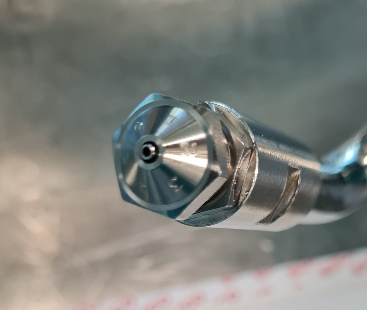
Figure 1: two-substance nozzle Schlick 970 S4 1.2 mm. Foto courtesy of Novartis AG.
A solution to this problem could be considering a larger gas orifice and imposing the desired air mass flow there. From a modelling perspective, this approach avoids resolving the spray atomization. However, it is necessary to properly consider the pressure at the simulation’s inlet in order to conserve the energy of the jet, see Figure 2.
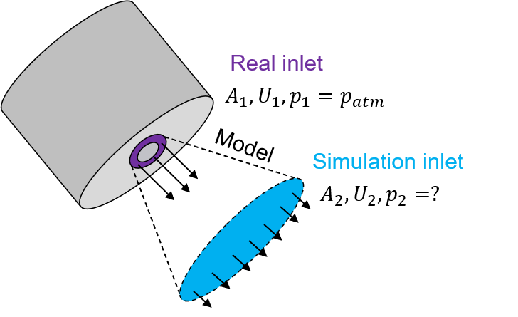
Figure 2: sketch showing the difference between real and simulation inlet boundary conditions.
If we assume the fluid to be incompressible and inviscid, the pressure at the (new) simulation inlet can be estimated using the Bernoulli equation as follows:
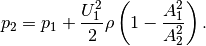
where  is equal to the atmospheric pressure. If the area of the simulation
inlet
is equal to the atmospheric pressure. If the area of the simulation
inlet  is ten times larger than the area of the nozzle’s orifice
  ,
then:
,
then:

The velocity boundary condition in the first equation ensures the same
mass flow as for the original nozzle, while the pressure boundary condition in the second
equation ensures the conservation of energy. In case of real spraying, the
dynamic pressure term needs to be scaled by a factor  to account
for energy losses through gas-liquid interaction, viscosity, non-adiabatic effects, etc..
Hence, the following modified Bernoulli equation is proposed:
to account
for energy losses through gas-liquid interaction, viscosity, non-adiabatic effects, etc..
Hence, the following modified Bernoulli equation is proposed:
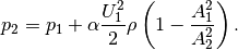
where  . This parameter is not known a priori and needs to be calibrated
by comparing simulation with experimental results.
. This parameter is not known a priori and needs to be calibrated
by comparing simulation with experimental results.
Continous voidfraction field across processor boundaries
With the divided voidfraction model voidfraction may be distributed across several cells. With the standard and engine locate models this distribution works only for cells on the same processor as the cell center and, thus, does not extend across processor boundaries. In most cases, especially for small particle to cell size ratios, the effect is small and the resulting jump in voidfraction upon the particle crossing from one processor to the next can be safely ignored.
In some cases, however, a smoother voidfraction might improve stability or overall acccuracy. There are two options to achieve this:
Use the engineIB locateModel which also provides information on particles close to processor boundaries to neighboring processors. This model is not restricted to resolved CFD-DEM simualtion but may also be used in unresolved simulations. Be aware that this model will incur a small performance penalty compated to the engine locateModel. To ensure particles close to processor boundaries are found on all neighboring processors, enlarge the processor bounding boxes by about one particle radius using the
bbOffsetparameter of the twoWaySocket data exchange model.Use the tetBased voidfraction model which inherently communicates particle contibutions to voidfraction across processor and cyclic boundaries without any further changes.
Use different particle shapes
See Spout bed for different particle shapes for a guide on different particle shapes in the same case setup.
(*) This offering is not approved or endorsed by OpenCFD Limited, the producer of the OpenFOAM software and owner of the OPENFOAM® and OpenCFD® trade marks.